Database Reference
In-Depth Information
for all
Thus, a particular point in the time series can be expressed as a linear combination
of the prior p values, for j = 1, 2, …p, of the time series plus a random
error term, . In this definition, the time series is often called a
white noise
process
and is used to represent random, independent fluctuations that are part
of the time series.
From the earlier example in
Figure 8.3
,
the autocorrelations are quite high for
the first several lags. Although it appears that an AR(8) model might be a good
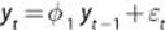
candidate to consider for the given dataset, examining an AR(1) model provides
further insight into the ACF and the appropriate value of p to choose. For an AR(1)
model, centered around
,
Equation 8.5
simplifies to
Equation 8.6
.
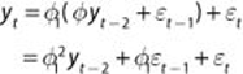
Based on
Equation 8.6
, it is evident that
. Thus, substituting
for
yields
Equation 8.7
.
Therefore, in a time series that follows an AR(1) model, considerable
autocorrelation is expected at lag 2. As this substitution process is repeated,
can be expressed as a function of for …and a sum of the error
terms. This observation means that even in the simple AR(1) model, there will be
considerable autocorrelation with the larger lags even though those lags are not
explicitly included in the model. What is needed is a measure of the autocorrelation
between for h = 1, 2, 3… with the effect of the values
excluded from the measure. The
partial autocorrelation function (PACF)
provides such a measure and is expressed as shown in
Equation 8.8
.
where