Cryptography Reference
In-Depth Information
1
1
2
3
4
5
6
7
8
9
10
11
12
13
14
15
16
0.8
0.6
0.4
0.2
0
2
3
4
5
6
7
8
9
10
T
g
(ns)
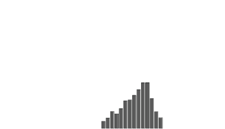
Fig. 18.7
Probability of number of error bytes for AES_PPRM1 module when the faults are injected
into the last round
area when the fault starts to be injected. This means that we can inject a fault into
almost the same bits between rounds 9 and 10 when we set
T
g
to the same length
as that of the starting point of the fault injection. Therefore, this figure shows that a
one-byte fault injected into any bit position of round 10 can also be injected into the
same position of the earlier round. Compared to the results of Fig.
18.8
a, the length
of the fragmented streaks is short and the number of errors of Fig.
18.8
b increases
when
T
g
<
8 ns when a clock glitch is generated in round 9. We conjecture that this
is because of the fault diffusion from the MixColumns operation in the AES block
cipher, which is not executed in the last round.
18.4.2 Experimental Results for Public Key Cryptography
This subsection presents the interrelation between the success probabilities of the
fault injection and the glitch width
T
g
for public key cryptography.
In these experiments, for RSA modules, a continuous 60-cycle clock glitch is
injected at a specific time during the computation of an RSA signature. For an ECC
module, a continuous ten-cycle clock glitch is injected at a specific time during an
ECC scalar multiplication. The detailed relationship between the success probabili-
ties of the fault injection and the glitch width
T
g
is shown in Fig.
18.9
. Each success
probability shown in Fig.
18.9
is produced from 1000 measurements. For each RSA
or ECC module, the success probability has been divided into 11 sections and shown
in different colors. For example, with
T
g
=
5 ns, no fault is injected for LR binary
with a dummy RSA module and the fault can be injected with probability of 0.1 for
the LR binary RSA module.
8
.