Adaptive Quasi-Linear Viscoelastic Modeling - Computational Modeling in Tissue Engineering - page 68

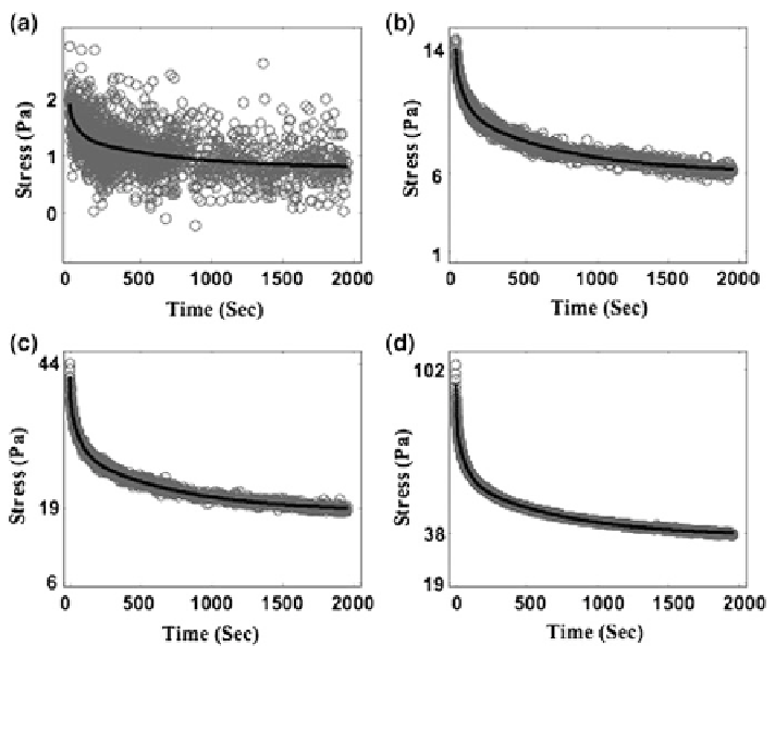
Fig. 6 Three time constant exponential fits (black curves) to hold-relaxation stress data (gray
circles) for the Adaptive QLV model. Optimum time constants: 5.5, 66 and 699 s. a Initial strain
of 0; b Initial strain of 0.0667; c Initial strain of 0.1333; d Initial strain of 0.2000

where

;

Þ ¼ 0 : 0667
20

e 20 = s i 1

c i 0 : 0667n ð k i 0 : 0667n ð Þ i ¼ 1 ; 2 ; 3 : ð 57 Þ

Therefore, the time constants s 1 , s 2 and s 3 could be calibrated simply by calibrating a
three time constant exponential function (with variable amplitudes) to all of the hold-
relaxation stress histories simultaneously. This is an interesting feature of the Adaptive
QLV model that simplifies the calibration significantly for exponential shape functions.
All four hold relaxation stresses were fitted with three-time constant expo-
nential curves by minimizing the integral I given in Eq. ( 48 ). The resultant fitted
curves (Fig. 6 ), with r o , c i and s i as shown in Table 1 , was an excellent fit of the
hold stress time history data in all four tests. The functions k i calculated for these
strains using Eq. ( 57 ) are listed in Table 2 . A cubic interpolation was used to
determine the r o and k i functions for strains from 0 to 0.2667 (Fig. 7 )[ 55 ].
Knowing the three parameters of the shape functions: s 1 , s 2 and s 3 , and r o and k i
functions for all strains the Adaptive QLV model was fully calibrated.