Random Processes - Random Signals and Processes Primer with MATLAB - page 388

where P X ( k ; t ) is the Poisson formula given in ( 6.71 ).
Similarly, the amplitudes of random variables X 1 and X 2 will have opposite
signs, if there are an odd number of zero crossings in the interval t :

PfX 2 ¼ UjX 1 ¼U ; tg¼PfX 2 ¼UjX 1 ¼ U ; tg
¼ 1
k¼ 1

(6.76)

P X ðk ; tÞ:

; 3 ; 5 ; ...

Finally, from ( 6.72 )to( 6.76 ), we get:

k k

1 1

l j t ðÞ l j t ðÞ

e ljtj U 2 e ljtj

R XX ðtÞ¼U 2

k ! k !

k¼ 0 ; 2 ; 4 ; ... k¼ 1 ; 3 ; 5 ; ...

" #

: (6.77)

k k

¼ U 2 e ljtj 1
k¼ 0

1

l j t ðÞ ljtðÞ

¼ U 2 e 2 ljtj

k ! k !

; 2 ; 4 ; ... k¼ 1 ; 3 ; 5 ; ...

Note that in the obtained result we have an absolute value of t because the time
interval t in the Poisson formula ( 6.71 ) is always positive, while in an autocorrelation
function time interval t takes all values from 1 until + 1 .
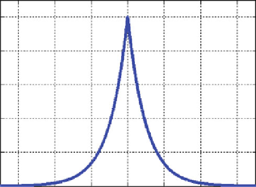
The autocorrelation function is shown in Fig. 6.10 for U ¼ 1 and l ¼ 0.5.
Next we verify the properties of the autocorrelation function for U ¼ 1:

P.1 The autocorrelation function has its maximum value at t ¼ 0, and it is equal to
U 2

¼ 1.

P.2 From ( 6.77 ), it is clear that the autocorrelation function is an even function,
i.e., R XX ( t ) ¼ R XX ( t ).

1

0.8

0.6

0.4

0.2

0

- 3 - 2 - 1 0 1 2 3

lt

Fig. 6.10 Autocorrelation function in Example 6.5.2