Digital Signal Processing Reference
In-Depth Information
a
b
1
0.4
0.35
1/16
0.9
1/4
0.8
0.7
0.6
0.5
0.3
0.25
3/8
0.2
0.4
0.3
0.2
0.1
0
−
0.15
0.1
1/4
0.05
1/16
0
1012
x
345 6
0
0.5
1
1.5
2
2.5
3
3.5
4
x
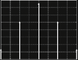
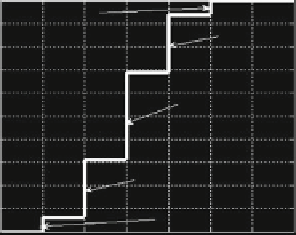
Fig. 5.15
Binomial distribution and density functions. (
a
) Distribution function. (
b
) Density
function
(a) It is necessary to find the probability that exactly two “1” pulses become “0.”
(b) Find the probability that no more than two false pulses appear (“0”s become
“1”). Plot the density function of the corresponding binomial random variables
which presents the number of false pulses.
Solution
(a) The number of lost “1” pulses in a code word is a binomial random variable in
which
n ¼
6 and
p ¼
0.04
q ¼
1
p ¼
1
0
:
04
¼
0
:
:
96
(5.125)
From (
5.109
), we have:
6
!
6
Þ¼C
6
p
2
q
4
04
2
0
96
4
PfX ¼
2
g¼P
X
ð
2
;
¼
0
:
:
¼
0
:
0204
:
(5.126)
2
!
4
!
The random variable
X
takes the discrete values
k ¼
0,
, 6, with the
...
corresponding probabilities
p
k
(1
p
)
nk
.
(b) The number of possible false pulses in the code word is also a binomial random
variable
X
in which
p ¼
0.1,
n ¼
4, and
k ¼
0, 1,
, 4. It follows that
...
q ¼
1
0.1
¼
0.9.
The probability that no more than two false pulses appear is given as:
4
g¼
X
2
C
4
0
1
k
0
9
nk
Pfk
2
:
:
¼
0
:
6561
;
k¼
0
þ
0
:
2916
þ
0
:
0486
¼
0
:
9963
:
(5.127)

Search WWH ::

Custom Search