Normal Random Variable - Random Signals and Processes Primer with MATLAB - page 244

a

b

LIN EA R TR A NSFO R MATIO N : Y=−3X+2 LINEAR TRANSFORMATION of NORMAL R.V.X

100 0.2

Y=−3X+2,

80 0.18

0.16

60

40 0.14

20 0.12 INPUT R.V. X

mX=−1, VA=4

0 0.1

−20 0.08

OUTPUT R. V. Y.

0.06

−40

mY=5; VA=36

−60 0.04

−80 0.02

0

−100

−30 −20 −10 0 10 20 30 −30 −20 −10 0 10 20 30 40

x,y

X

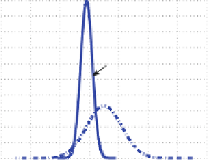
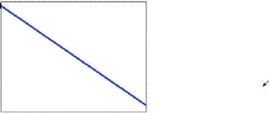
Fig. 4.7 Linear transformation of a normal random variable. ( a ) Linear transformation. ( b ) Input
and output PDFs

Figure 4.7a shows the transformation and Fig. 4.7b shows the input and the
transformed PDFs.

4.3.1.2 Nonlinear Transformation

We use the expression ( 2.138 ) to illustrate that the nonlinear monotone transforma-
tion of a normal variable does not result in a normal variable.

Example 4.3.2 In this example, consider the logarithmic transformation

Y ¼ e X

(4.77)

of a normal variable with parameters m X and s X .
The transformed PDF according to ( 2.138 ) is:

e ð ln y m X Þ 2

f X ð x Þ
d d x

1
2 p

2 s 2
X

f Y ðyÞ ¼ ¼ p y> 0 (4.78)

;

x¼ ln y

s X y

The obtained PDF is lognormal and will be examined in more detail in the next
chapter. The transformation as well as input and output PDFs are shown in
Fig. 4.8a , b, respectively.

4.3.2 Nonmonotone Transformation

The nonmonotone transformation of a normal random variable changes the variable
such that the resulting variable is not normal, as shown in the following example.

Example 4.3.3 We consider the absolute value of the normal variable with a zero
mean value and a variance of 1.