Graphics Reference
In-Depth Information
region, it is not seen. Sometimes we can do
beter. In the previous chapter, we showed
that we could create an analytic height-
field function surface with a vertex shader,
computing the normal at each vertex by
using partial derivatives. We can also cre-
ate the normals at each pixel in a fragment
shader by the same technique.
We begin by interpolating the points
in the horizontal plane of the function in
the rasterizer. It is straightforward to get
these from the
aVertex
values in the ver-
tex shader, and then create a
vec2
varying
variable for the fragment shader's use. You also need to pass the actual pixel
position as a varying variable, because that is needed in the
ADSLightModel( )
function. You then compute the normal from the interpolated domain coordi-
nates and pass that value and the position to the lighting function to get the
pixel color.
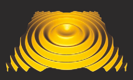
The result is shown in Figure 8.7, which should be compared with
Figure 7.7 in the previous chapter. Notice how much more smoothly this sur-
face moves from one primitive to another, especially in the area along each of
the foreground ridges. Is this beter than Phong shading? Theoretically, yes,
because it is analytic. Visually, it will probably depend on the nature of the
surface. This is explored in an exercise.
The fragment shader for this figure is shown below. It uses the
ADSLightModel( )
function given above, so that function has been abridged.
The surface is given by the function
fxy
Figure 8.7.
The rippled surface with exact shading.
(
)
2
2
(, )
=∗ +
03
.
sin
x
y
with partial
derivatives
∂
∂
∂
∂
f
x
(
)
2
2
=
203
.* .
∗ ∗
x
cos
x
+
y
,
f
y
(
)
=
203
.* .
∗ ∗
y
cos
x
2
+
y
2
.
You will see these in the fragment shader code below, where we assume
that the two input variables
vMyXY
and
vPos
come from a vertex shader.
in vec2 vMyXY;
in vec4 vPos;
out vec4 fFragColor;