Biology Reference
In-Depth Information
30
20
10
0
-
10
-
20
-
30
-
40
-50
-45
-40
-35
-30
-25
-20
-15
-10
-5
0
First component
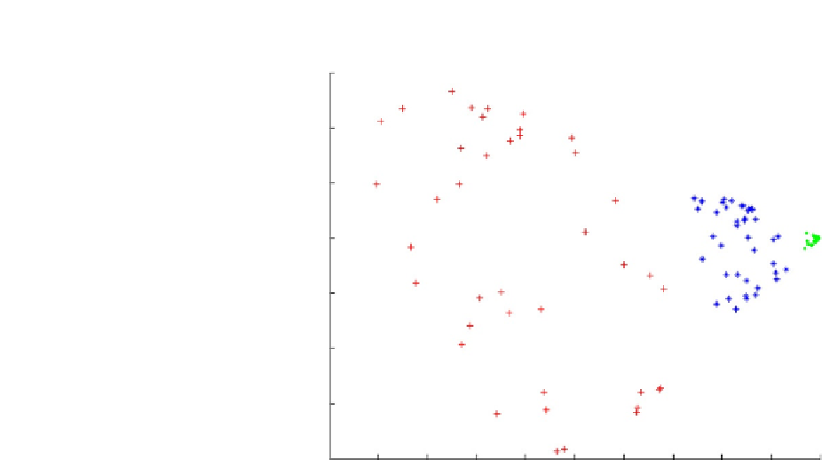
FIGURE 2.6
Output of a PCA. The first principal component is plotted against the second principal
component, and different categories of case are indicated by colour. Image courtesy of Petter
Strandmark, via Wikimedia Commons.
25
individual cases and the columns are the variables associated with the cases. These
variables are usually inter-correlated. The aim of PCA is to extract the important
information from the matrix and present it as a set of new orthogonal variables,
the
principal components
, created by combining the existing variables. The principal
components explain the variability in the data. Optimally, the first few principal
components will explain most of the variability, and the rest of the principal com-
ponents can be discarded. Further analysis can then be carried out using just a small
number of principal components, instead of a large number of original variables. The
mapping between the original matrix of variables and the principal components can
be used to compute factor scores for new cases as they arise. The relationship
between individual cases and the principal components can be visualised by display-
ing them as points on maps (
Figure 2.6
)(
Abdi and Williams, 2010
).
PCA has contributed to the analysis of large datasets in just about every aspect
of microbiology. Some interesting recent applications include investigation of
metagenomes in the human gut, both normal (
Qin
et al.
, 2010; Wu
et al.
, 2011
)