Modeling of Flight Delay State-Space Model - Advanced Research on Computer Education, Simulation and Modeling - page 28

α = ∑ ) is the

m

Where Θ =( α i ,…, α m , θ 1 ,…, θ m ) is the parameter vector, α j ( α j ∈ [0,1],

j

j=1

ψ j (r i ⏐θ j ) is the density function of jth compo- mixing weight of jth component, and

nent depending on parameter θ j . In this paper, we assume that g is a normal mixture

j is denoted as j =( j , ∑ j ), where

denotes the mean and ∑ denotes the

model. And θ θ μ μ

covariance matrix.

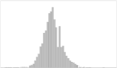
0.1

0.08

0.06

0.04

0.02

0

-0.6 -0.4 -0.2 0 0.2 0.4 0.6

Rate

Fig. 1. Density Distribution of Original Delay Rate

2.3 Parameter Estimation Based on Genetic EM Algorithm

EM algorithm is the most popular and effective method for parameter estimation.It is
an iterative two-step procedure: E-step and M-step. The E-step calculates the expecta-
tion of the log likelihood on the observed data R and the current value of

Θ . The M-

step updates the corresponding estimate of Θ . After a certain number of iterations, the

algorithm obtains the local optimal value of . In order to avoid the local maximum

problem associated with the traditional EM algorithm, ideals of GA can be applied to
EM to find the global optimum. The combination of GA and EM is known as genetic
EM algorithm [6]. The procedure of the genetic EM algorithm is shown as following.
Initial: oldChrom, Emrate,bestFit,oldFit;
while (bestFit-oldFit) > EMRate
fitV = Evaluation (oldChrom,R);
newChrom = Selection(oldChrom, fitV,ps);
newChrom = Crossover(newChrom, k, pc);
newChrom = Mutation(newChrom, pm);
newChrom = EM(newChrom,R);
oldFit = bestFit;
bestFit = max(fitV);
newChrom = sortByMiu(newChrom);
oldChrom = newChrom;
end
The fitness function used in the genetic EM algorithm is the log likelihood function

Θ

of defined in equation (5) and calculation stops when improvement of the fitness

function value decreases below a given threshold.

Θ