Biomedical Engineering Reference
In-Depth Information
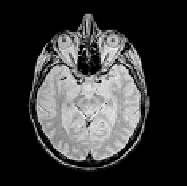
(a)
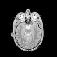
(b)
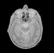
(c)
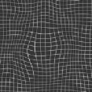
(d)
Figure 9.10:
The reference (a) and test (b) images with superimposed land-
marks (in red). The superimposed images after registration using the semi-
automatic algorithm (c) and the deformation field found (d). Corresponding
anatomical structures are well identified; the alignment is clearly superior to
that in Figure 9.9. (Color slide.)
9.4.8.1
Explicit Derivatives
For the optimization algorithm, we need to calculate the partial derivatives of
E
, as they form the gradient vector
∇
c
E
(
c
(
i
)
) and the Hessian matrix
∇
c
E
(
c
(
i
)
).
2
Starting from Eq. (9.7), we obtain the first partial derivatives
∂
E
∂
c
j
,
m
=
x
=
g
(
i
)
∂
g
m
(
i
)
∂
f
w
(
i
)
∂
f
t
(
x
)
1
I
∂
e
i
(9.12)
∂
x
m
∂
c
j
,
m
i
∈
I
b
as well as the second partial derivatives
∂
∂
g
m
2
E
∂
c
j
,
m
∂
c
k
,
n
=
∂
f
w
(
i
)
2
∂
f
t
2
e
i
∂
x
m
∂
f
t
2
f
t
∂
x
m
∂
x
n
1
I
∂
e
i
∂
c
j
,
m
∂
g
n
∂
∂
f
w
(
i
)
∂
(9.13)
∂
x
n
+
∂
c
k
,
n
i
∈
I
b
∂
f
w
(
i
)
=
2
f
w
(
i
)
−
f
r
(
i
)
and
From (9.7) defining the SSD criterion, we get
∂
e
i
2
e
i
∂
f
w
(
i
)
2
∂
=
2. The derivative of the deformation function (9.10) is simply
∂
g
m
∂
c
j
,
m
=
β
n
m
(
x
/
h
−
j
)
. The deformation model is linear and all its second derivatives
are therefore zero; that is the reason for the simplicity of (9.13). The partial