Faulted Surfaces - 3-D Structural Geology - page 219

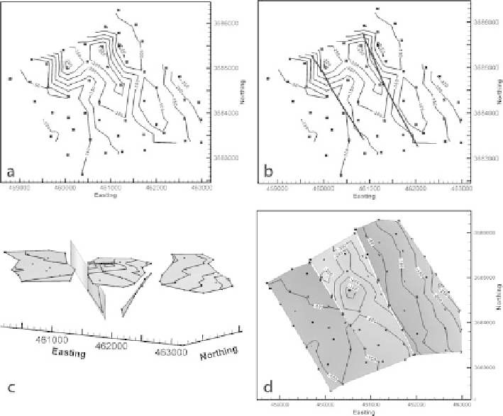
Fig. 8.6. Example of procedure for fault interpretation applied to top of Gwin coal cycle, Deerlick Creek
coalbed methane field, Alabama (based on data in Groshong et al. 2003b). Contour interval is 50 ft, squares
show well locations. a Top of the Gwin contoured without faults. b Top of the Gwin showing approximate
fault traces. c 3-D oblique view of top Gwin broken into separate blocks at fault traces and re-contoured.
d Top of Gwin re-mapped to fit the faults. Additional squares are points defining HW and FW cutoff lines
footwall blocks (Fig. 8.6c) and finally re-mapped to join the marker surface to the fault
planes (Fig. 8.6d). The final re-mapping requires contouring up to and across the fault
planes and must honor the known fault separations. Locating the faults, projecting
beds to the fault surface, and contouring up to and across a fault will be discussed next.
8.3.1
Locating the Fault
In mapping a single marker surface with data from wells, the exact location of a fault
is usually uncertain. Closely spaced, parallel contours on the marker surface provide
a clue to the presence of a fault but do not necessarily give an accurate location. For
example, the traces of the faults in Fig. 8.6b are in regions of closely spaced contours
but do not follow the contours. Furthermore, it is rare for a well to cut a fault exactly at the
marker horizon being mapped and so direct evidence of the fault location in the marker
horizon is usually absent. All fault cuts at any stratigraphic level that can be correlated