Graphics Reference
In-Depth Information
TABLE 3.2
Parameters of ARX Model in Experiment 1
Parameter
Calculation
A(q)
1 - 2.444 q
-1
+ 2.001 q
-2
- 0.5565 q
-3
+ 4.21e - 006 q
-4
+ 0.1708 q
-5
- 0.4541 q
-6
+ 0.2823 q
-7
B(q)
-2.375 × 10
-7
q
-1
+ 3.072 × 10
-7
q
-2
- 2.84 × 10
-7
q
-3
- 3.156 × 10
-7
q
-4
- 1.18 × 10
-7
q
-5
+ 1.263 × 10
-6
q
-6
- 6.156 × 10
-7
q
-7
Operating point
u = 1.5331 × 10
5
, y = 98.261
Measured and Simulated Output
18
16
14
12
10
Measured output
Simulated output
8
6
0
1000
2000
3000
4000
5000
6000
7000
8000
9000
10,000
×10
6
2.2
2
1.8
1.6
1.4
1.2
1
0.8
0.6
0
1000
2000
3000
4000
5000
6000
7000
8000
9000
10,000
Frame
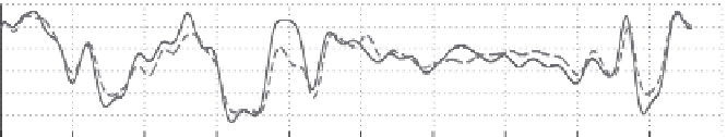
FIGURE 3.9
Error between measured and simulated output of application in Experiment 1.
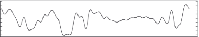
more difficult as shown in the varying output levels compared to the first experi-
ment. The actual data captured consist of more spikes due to interruptions from
other computer processes and the data must be filtered so that a reasonable model
can be derived. Nevertheless, through the proposed approach, we are able to obtain
a system model that produced output with an error less than 4 FPS. The parameters
of this model are presented in Table 3.3.
3.6.2 e
xPeRiment
2
We extended our modelling framework for rendering to consider more than one
input. Based on selected combinations of two input variables (vertex count and
shader value), we generated steady-state output responses of three settings as shown
in Figure 3.10. Each graph in the figure indicates the steady-state input-output rela-
tionship exhibited by the system based on a certain combination of the values of the
two inputs. The profiles of the measured inputs and outputs of the actual rendering
are shown in Figure 3.11. A comparison of the simulated model and the measured


Search WWH ::

Custom Search