Database Reference
In-Depth Information
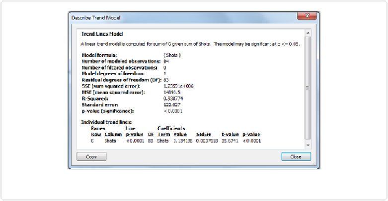
The equation tells us that the line has a slope of 0.134198, meaning that for every increase of
one shot (along the x-axis), the line rises 0.134198 units (along the y-axis). The p-value in-
dicates that there is a very small chance (< 0.0001, or < 0.01%) that two variables without
any correlation at all would produce such a relationship. They are definitely correlated, and
this comes as no surprise.
But how good is the fit? We can find that and much more by right-clicking on the trend line
and selecting
Describe Trend Model
. The window shown in
Figure 8-19
appears.
Figure 8-19. Describe Trend Model window
From this window, we can see a number of different aspects of the model, including its coef-
ficient of determination (R-Squared) and its Standard error. Since we forced the trend line to
cross the y-axis at y=0, we can't use the R-Squared value in the typical way, namely, to un-
derstand how well the model fits the data. Try editing the trend line by unchecking the
“Force y-intercept to zero” box and then choose “Describe Trend Model” once again. You'll
notice that the R-Squared value drops from 0.938774 to 0.302579.
The line divides the grid area into two sections. The data points that lie above and to the left
of the upward sloping line can be thought of as having higher accuracy: it took these players
fewer shots to achieve a certain number of goals, as compared to the model. The data points
that lie below and to the right of the line can be though of in the opposite way: it took a relat-