Geology Reference
In-Depth Information
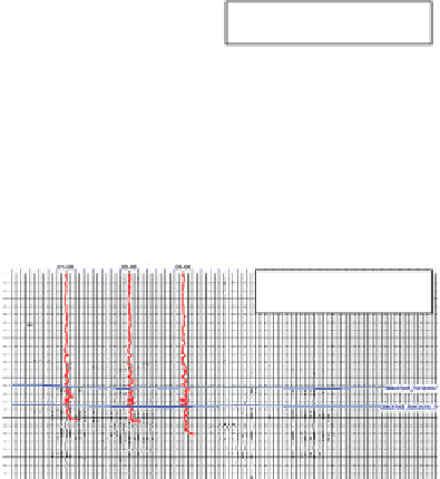
Note the good fit at the reservoir target at 1.75 s and the
poorer fit below, related to the presence of multiple
energy in the seismic.
Two separate aspects of the inversion can be
checked through comparisons of inverted and logged
impedances at wells. Firstly, the scaling of the wavelet
can be investigated. If the wavelet scaling is correct
then the excursions of impedance around the low-
frequency trend should be similar in amplitude for
the well data and the impedance result. This scaling is
derived from the well ties and might need adjustment
if the ties have to be carried out over a different
stratigraphic interval or depth range to the inversion
target. Secondly, the goodness of fit of the inverted
impedance and the logged impedance is to some
degree dependent on the frequency cut-off applied
to the low-frequency model. As the cut-off frequency
is made lower, the inverted impedance is likely to give
a worse fit. It should be remembered that a good fit at
the wells does not ensure that the inversion is good
away from the wells. There may be biases for example
introduced by lateral variations in the low-frequency
component.
A display of the difference between the input
reflectivity section and the synthetic section calcu-
lated from the inverted impedance, using the inver-
sion wavelet, is also a useful display for quality
control. Ideally the display should have very low
amplitudes everywhere with no coherent energy
(
Fig. 9.10
). High amplitudes on the error display
may be caused by the inverted impedance hitting a
constraint boundary. This display can also be used to
evaluate the best frequency cut-off for the back-
ground model. As the cut-off is made higher, the
synthetic error is likely to increase. Of course, because
of non-uniqueness, a small error does not guarantee
the right answer. There are an infinite number of
impedance volumes that will match the reflectivity
input data.
a)
Input seismic
800
900
1000
1100
1200
b)
Inversion synthetic
800
900
1000
1100
1200
c)
Inversion error
800
900
1000
1100
1200
Figure 9.10
Input seismic compared to synthetic generated from
inverted impedances; (a) input seismic, (b) synthetic generated from
inversion, (c) difference between (a) and (b). Courtesy CGGV
Hampson-Russell Software and Services.
9.2.4.1 Background model
The illustration in
Fig. 9.11a
shows a sparse spike
inversion result (Francis and Syed,
2001
). Applying
a low-pass filter reveals the background model
(
Fig. 9.11b
). It is clear that the pinchout in the final
inversion result is quite simply a result of the back-
ground model. Applying a bandpass filter to the
inversion result and comparing it with bandlimited
impedance from seismic (
Chapter 5
) will reveal how
much additional information is provided by the abso-
lute inversion (e.g. Francis and Syed,
2001
; Lancaster
and Whitcombe,
2000
). Often, the two bandlimited
impedance products look identical.
9.2.4 Inversion issues
Often interpreters are not involved in the process of
creating an inversion but it is their job to interpret it.
Prior to applying geological thought to the inversion
products it is necessary to evaluate as best as is pos-
sible the usefulness of the inversion. There are a
number of distinct issues related to the low-frequency
component and the wavelet of which the interpreter
should be aware.
9.2.4.2 Low-frequency merge
A particular issue with seismic inversion is the
merging of the low-frequency component. Wagner
204