Geology Reference
In-Depth Information
a)
P-Impedance
(m/
s
.g/cc)
2.05
AI (ft/s.g/cc)
5000
2.1
1600
43000
2.15
5500
41100
2.2
39200
1800
6000
2.25
37300
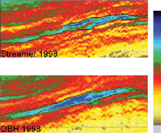
Streamer 1998
35400
2000
33500
6500
31600
2.05
29700
7000
2200
2.1
27800
25900
2.15
7500
24000
2.2
2400
8000
undefined
2.25
OBH 1998
AI (ft/s.g/cc)
b)
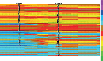
Figure 9.12
Comparison of inverted seismic sections from surface
streamer and ocean-bottom hydrophone, after Wagner
43000
et al.
,
2006
.
1700
41100
39200
37300
1900
are observable differences in the inversion. In the
extreme case where the true phase of the seismic
wavelet is 90° different from that used in the inver-
sion, a step change in impedance will become trans-
formed into a thin bed in the inverted result. The
accuracy to which wavelet phase needs to be known
will vary depending on the data and what the inver-
sion result will be used for, but in general an accuracy
of 30° or better is needed.
Figure 9.16
shows an
example of how an error in phase of 45° can influence
the inversion result. Assuming that the impedance of
the upper layer is matched, the error in phase changes
the general scaling of the impedances although the
general form is similar. It is evident that an accurate
appreciation of wavelet shape and scaling (
Chapter 4
)
is invaluable in deriving a good inversion.
When several wavelets are available from different
well ties, they can be averaged provided their ampli-
tude and phase characteristics are similar (
Fig. 9.17
).
Usually the wavelets would be aligned on the domin-
ant peak or trough before averaging, to allow for
small static shifts arising from errors in the time
35400
33500
2100
31600
29700
27800
2300
25900
24000
Figure 9.11
An example of a background model adversely
influencing a broadband inversion result; (a) model-based inversion,
(b) starting model based on interpolation of well data. The pinch-out
is located halfway between the wells because of the interpolation
methodology used (after Francis and Syed,
2001
).
et al. (
2006
) highlighted the problem of merging the
low frequency with a sparse spike inversion result in a
comparison of inversions from streamer and ocean-
bottom hydrophone (OBH) data. A key issue for these
datasets is the difference in frequency content, with
the streamer data having a reduced range of frequen-
cies compared to the OBH. A comparison of the
inversion results from the two surveys shows signifi-
cant differences, with the streamer data showing
apparently greater resolution with more layers evident
in the reservoir section (
Fig. 9.12
). However, it is
probable that the apparent layering in the streamer
data is related to residual effects from the bandlimited
impedance. The low frequency has not been correctly
merged. The wedge model in
Fig. 9.13
illustrates the
problem. Maps of the impedance results from time-
lapse data show dramatic differences between the
streamer and OBH data (
Fig. 9.14
).
-
depth relations. This of course requires the wavelets
to have a similar general appearance.
Wavelet averaging would not be the correct thing
to do if the wavelet varies systematically either lat-
erally or with depth. As discussed in
Chapter 5
, vari-
ation in both frequency content and phase with depth
is to be expected; lateral variation is also possible, for
example due to lateral change in absorption. In many
cases the variation in depth of the target zone is small
across the area of the inversion study, so its effect on
the wavelet can generally be ignored. However, lateral
variation can be quite significant, for example if there
are localised patches of gas-filled sands
9.2.4.3 Wavelet issues
Understanding the wavelet in the data is essential for
deriving reliable inversions.
Figure 9.15
shows how
inversion can be very sensitive to the wavelet used.
Although the wavelets shown are very similar there
205
in the