Geology Reference
In-Depth Information
9.8
a)
1
9.6
0.5
9.4
0
9.2
-0.5
9
-1
8.8
-90
-60
-30
0
30
60
90
χ
GR
S
w
8.6
8.6
8.8
9
9.2
9.4
9.6
9.8
b)
GR (API)
EEI(-51)
S
w
(dec)
EEI(25)
LnAI
0
150
0
12000
1
0
5000
10000
gas sands
wet sands
shales
carbonates
Figure 5.63
The AI/GI crossplot.
9
8.9
Gas sand
Oil sand
Brine sand
8.8
20m
8.7
8.6
8.5
8.5
8.6
8.7
8.8
8.9
9
LnAI
Figure 5.64
angle from averaged log data
using the method described by Whitcombe and Fletcher,
2001
.
Determination of fluid
χ
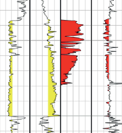
Figure 5.65
Correlation of EEI with gamma ray and water
saturation logs; (a) correlation diagram showing maximum
correlations at 25° and 51° for water saturation and gamma ray
respectively, (b) log plot showing comparisons of EEI (χ ¼51°) with
gamma ray and EEI
(
Fig. 5.65a
). The log plots in
Fig. 5.65b
show the
sand defined on the EEI(
51°) log and the pay zone
(χ ¼ 25°) with water saturation.
on the EEI(25°) log.
Similarly the correlation technique shows that
certain
angles correlate strongly with particular
angle independent elastic properties (
Fig. 5.66
)
(Whitcombe et al.,
2002
). Numerous authors
(such as Dong,
1996
) had observed that certain
combinations of intercept and gradient relate
to changes in particular elastic parameters but
the idea of AVO projections and the EEI formula-
tion is
χ
Perhaps a more geological approach is to analyse
EEI in terms of lithological and fluid related facies.
Figure 5.67
illustrates the idea with shales, water
sands and oil sands defined from well logs. The degree
of discrimination can be appreciated by using histo-
gram displays with simple Gaussian fits and inter-
actively changing
angle.
It should be noted that there is not always a
lithology angle at a high angle to the fluid projection.
χ
an elegant way of
illustrating these
relationships.
102