Geology Reference
In-Depth Information
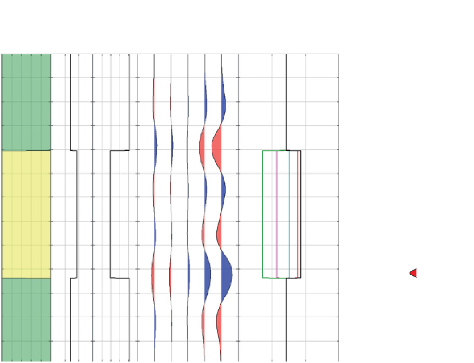
Lith
AI
PR
Gather
EI
4
7 0
0.5
0º 10º20º
30º
40º
4
7
(2 term) EI Legend
0º
10º
20º
30º
40º
AI
=
Figure 5.62
The relationship between reflectivity and elastic impedance.
2
4
0
@
1
A
0
@
1
A
0
@
1
A
3
5
ð
p
q
r
(GI) (gradient impedance) replacing gradient
reflectivity. Elegantly, the AI vs GI crossplot main-
tains the same angular relationships as the intercept
vs gradient crossplot, and an example is shown in
Fig. 5.63
.
There are a number of ways of calculating
V
p
V
p0
ρ
ρ
0
V
s
V
s0
EEI
ðÞ¼
V
p0
ρ
0
5
:
23
Þ
where
p
¼
cos
χ
+ sin
χ
,
angles
from EEI data.
Figure 5.64
shows the determination
of the fluid angle from averaged log data from sands
with various fluid fill (Whitcombe and Fletcher,
2001
).
Note that
χ
¼
χ
q
8k sin
and
r
¼
cos
χ
4k sin
χ
.
EEI effectively encompasses EI,soitcanbecon-
sidered the more general treatment for two-term
angle-dependent impedance. Given that EEI is
driven by the AVO crossplot angle it follows that
EEI (
χ
angles can also be calculated by
correlating EEI
logs
(calculated from +90°
to
90°) with fluid and lithology logs. For example,
Fig. 5.65
shows the correlation of a gamma ray and
water saturation (S
w
)logwithEEI.TheS
w
log
shows
90° is the impedance related to gradient
reflectivity and is appropriately called gradient
impedance (GI). Given the logarithmic relationship
of reflectivity and impedance (
Eq. (2.2)
)theAVO
crossplot can effectively be re-drawn with ln(AI)
replacing R
0
(zero incidence reflectivity) and ln
χ
)
¼
a maximum positive
correlation with
EEI(25°) whilst
the
gamma
ray
log has
a
maximum negative correlation with EEI(
51°), typ-
ical values for fluid and lithology angles respectively
101