Information Technology Reference
In-Depth Information
and
is the harmonic perturbation. Note that the autocorrelation for the network
response is given by (
7.72
) and the linear response function is given by (
7.73
).
In the specific case of a harmonic perturbation (
7.82
), after some straightforward
algebra, we obtain from (
7.93
)for
t
ξ
p
(
t
)
→∞
g
0
g
0
+
ω
(
t
)
=
ε
2
[
g
0
cos
(ω
t
)
+
ω
sin
(ω
t
)
]
,
(7.96)
which can be written in the more compact form
g
0
g
0
+
ω
(
t
)
=
ε
cos
(ω
t
−
φ),
(7.97)
2
1
/
2
with the phase defined as
arctan
g
0
ω
φ
=
.
(7.98)
The measure of stochastic resonance is typically the signal-to-noise ratio. We note
that the coefficient
D
in (
7.86
) is the measure of the noise intensity. In the unperturbed
case the coupling coefficient is given by (
7.89
). Let us assume, for simplicity's sake,
that
R
=
1 and
Q
0
=
1, which yields for the strength of the noise
1
=
g
0
)
.
D
(7.99)
ln
(
1
/
One measure for the visibility of the signal in the noise background is given by the
signal-to-noise intensity ratio, which in this case is given by the amplitude in (
7.97
):
ln
1
g
0
ε
S
D
=
g
0
g
0
+
ω
.
(7.100)
2
1
/
2
Consequently, when the intensity of the noise vanishes,
D
=
0, then so does the cou-
pling coefficient
g
0
=
0, and, consequently the signal-to-noise ratio does too,
S
/
D
=
0.
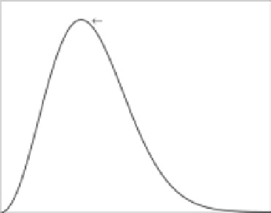
Stochastic-resonance peak
Noise magnitude
The signal-to-noise ratio for a generic stochastic-resonance process is depicted as a function of
the noise magnitude. It is clear that the signal-to-noise ratio is non-monotonic and achieves a
maximum for some intermediate value of the noise magnitude.
Figure 7.6.