Partial Least Squares Modeling of Lunar Surface FeO Content with Clementine Ultraviolet-Visible Images - Planetary Exploration and Science: Recent Results and Advances - page 14

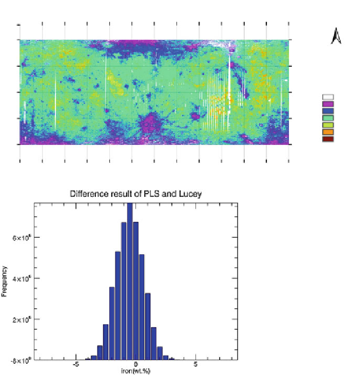
a Difference map of PLS model and Lucey 2000

120º 0'0”W 90º 0'0”W 60º 0'0”W 30º 0'0”W 150º 0'0”W 0º 0'0” 30º 0'0”E 60º 0'0”E 90º 0'0”E 120º 0'0”E 150º 0'0”E 180º 0'0”

N 180º 0'0”

70º 0'0”N

70º 0'0”N

35º 0'0”N

35º 0'0”N

FeO wt.%
-6.9--4.6
-4.5--2
-1.9--1
-.9-1
1.1-1.9
2-4.9
5-17.8

0º 0'0”

0º 0'0”

35º 0'0”s 35º 0'0”s

70º 0'0”s

70º 0'0”s

180º 0'0” 150º 0'0”W 120º 0'0”W 90º 0'0”W 60º 0'0”W 30º 0'0”W 0º 0'0” 30º 0'0”E 60º 0'0”E 90º 0'0”E 120º 0'0”E 150º 0'0”E 180º 0'0”

b

Fig. 1.10 ( a ) Difference map between iron map derived from PLS model and Lucey's algorithm
(PLS minus Lucey's). ( b ) The difference of the two maps shows a Gaussian distribution with an
average of 0.27 wt%, and RMS is 1.13 wt%

around 17 wt%. Comparing from the statistical results (Fig. 1.9 ), FeO abundance
derived by PLS model in lunar highland areas is a little higher than Lucey's but is
similar to LP's. Detail comparisons between PLS model, Lucey's algorithm, and LP
result will be discussed in the following.
In order to show the global difference between PLS model and Lucey's method,
we apply Lucey's algorithm to Clementine DIM and make a difference map (PLS
FeO minus Lucey's FeO), as shown in Fig. 1.10a . Most of the difference distributes
within 0.9 to 1.0 wt% which is shown in green color in the difference map. PLS
model gets an even higher iron abundance than Lucey's result in lunar farside,
which is consistent with the statistical result comparison (Fig. 1.9b, c ). Another