Graphics Programs Reference
In-Depth Information
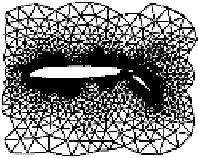
clf
gplot(A,[x y])
axis off
(Try zooming in on this plot by typing
zoom
and dragging the mouse.)
The adjacency matrix here (
A
) is a 4251
4253 sparse matrix with 12,289
non-zero elements, occupying 164 kB of storage. A full matrix of this
size would require 145 MB.
(From now on in this topic, the
clf
command will be omitted from
the examples; you will need to supply your own
clf
s where appropriate.)
×
25.2 Example: Communication Network
Suppose we have a communications network of nodes connected by wires
that we want to represent using sparse matrices. Let us suppose the
nodes are 10 equispaced points around the circumference of a circle.
dt = 2*pi/10;
t = dt:dt:10*dt;
x = cos(t)';
y = sin(t)';
plt(x,y)
axis equal off
for i = 1:10
text(x(i),y(i),int2str(i))
end
We want the communications channels to go between each node and its
two second-nearest neighbours, as well as to its diametrically opposite
node. For example, node 1 should connect to nodes 3, 6, and 9; node 2
should connect to nodes 4, 7, and 10; and so on. The function
spdiags
is used on the following to put the elements of
e
along the second, fifth,
and eighth diagonals of the (sparse) matrix
A
. If you look at the help for
spdiags
, you should be able to follow how these statements define the
connection matrix we want. First we define the connection matrix:
e = ones(10,1);
A = spdiags(e,2,10,10) + ...
spdiags(e,5,10,10) + ...
spdiags(e,8,10,10);
A=A+A';
Now do the plot: