Graphics Programs Reference
In-Depth Information
25.1 Example: Airfoil
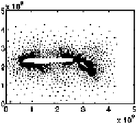
Suppose we are doing some finite element modelling of the airflow over
an aeroplane wing. In finite element modelling you set up a calculation
grid whose points are more densely spaced where the solution has high
gradients. A suitable set of points is contained in the file
airfoil
:
load airfoil
clf
plot(x,y,'.')
There are 4253 points distributed around the main wing and the two
flaps. In carrying out the calculation, we need to define the network of
interrelationships among the points; that is, which group of points will
be influenced by each point on the grid. We restrict the influence of
a given point to the points nearby. This information is stored in the
vectors
i
and
j
, included in the loaded data. Suppose all the points are
numbered 1
,
2
,... ,
4253. The
i
and
j
vectors describe the links between
point
i
and point
j
. For example, if we look at the first five elements:
>> [i(1:5) j(1:5)]'
ans =
1
2
3
5
4
2 310 10 11
The interpretation is that point 1 is connected to point 2, point 2 is
connected to point 3, points 3 and 5 are connected to point 10, and so
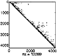
on. We create a sparse adjacency matrix,
A
, by using
i
and
j
as inputs
to the
sparse
function:
A = sparse(i,j,1);
spy(A)
The
spy
function plots a sparse matrix with a dot at the positions of
all the non-zero entries, which number 12,289 here (the length of the
i
and
j
vectors). The concentration of non-zero elements near the diagonal
reflects the local nature of the interaction (given a reasonable numbering
scheme). To plot the geometry of the interactions we can use the
gplot
function: