Graphics Programs Reference
In-Depth Information
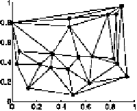
diagram. Such a triangular grid can be calculated
for our seamount example of the last section. The
triangles are defined using the
delaunay
function:
>> tri = delaunay(x,y);
>> tri(563:end,:)
ans =
2 4 7
1 2 6
8 3 11
25 245 59
We have displayed the last few lines of the
M
3 matrix
tri
, which
defines the triangles by a set of triplets that are indices into the
x
and
y
vectors. For example, the four triangles we have displayed in
ans
are
1:
x
(2)
,y
(2)
x
(4)
,y
(4)
x
(7)
,y
(7)
2:
x
(1)
,y
(1)
x
(2)
,y
(2)
x
(6)
,y
(6)
3:
x
(8)
,y
(8)
x
(3)
,y
(3)
x
(11)
,y
(11)
4:
x
(25)
,y
(25)
x
(245)
,y
(245)
x
(59)
,y
(59)
×
We can use this triangulation matrix to plot a surface of the seamount
data; each face of the surface is one of the triangles:
trisurf(tri,x,y,z)
hold on
plot3(x,y,z,'o')
axis tight
The functions
trisurf
and
trimesh
do not create surface objects;
rather, they create
patch
objects.
37 Three-dimensional Modelling
37.1 Patches
In this section we discuss the representation of real-world objects. Such
objects are built up using their faces (the six faces of a cube, for exam-
ple). In matlab “faces” are patches, and are defined using the
patch
command. Patches are blobs of coloured light (or ink) that are defined by
vertex points. The line between the vertices is the patch's
edge
and the
enclosed area is the patch's
face
. Before talking about three-dimensional
objects we discuss the simpler two-dimensional patch.