Geology Reference
In-Depth Information
1000
800
600
400
L
A, B
200
C
1
P
1
P
2
Fig. 8.40
The half-Schlumberger electrode configuration.
See Question 4.
100
80
60
40
C, D
that as
L
(the current electrode half-separation)
increased a CST was built up.
R
represents the re-
sistance measured by the resistivity apparatus.
20
10
1
2
4
6
8 10
20
40 60 80 100
200
a
(m)
L
(m)
R
(
W
m)
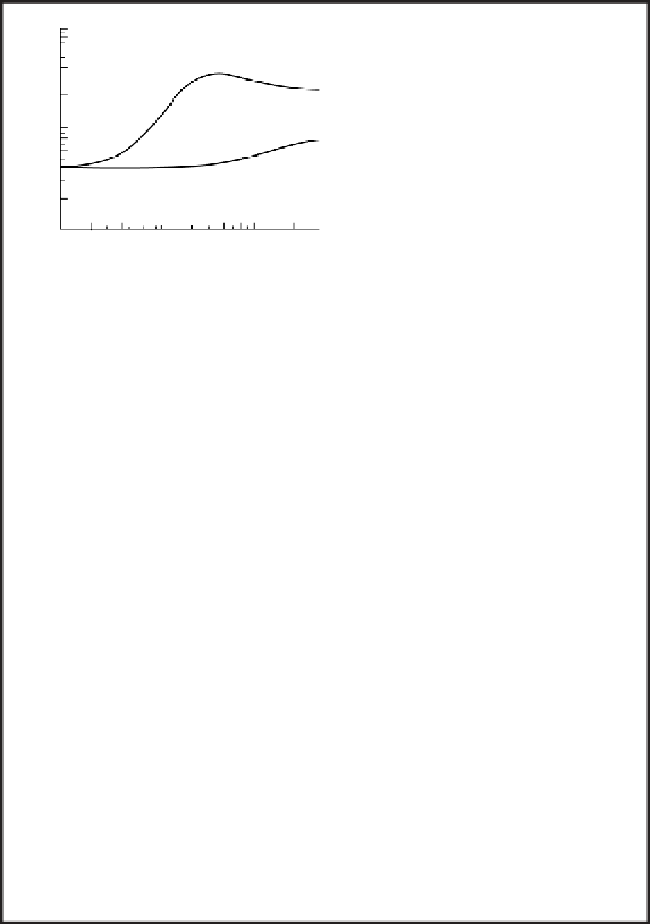
Fig. 8.39
Wenner VES sounding data for the locations shown
in Fig. 8.38.
30.2
1244.818
53.8
255.598
80.9
103.812
A seismic refraction line near to D revealed 15 m
of drift, although the nature of the underlying
basement could not be assessed from the seismic
velocity.
(a) Interpret the geophysical data so as to pro-
vide a geological section along the profile.
(b) What further techniques might be used to
confirm your interpretation?
(c) If a CST were to be performed along the
profile, select, giving reasons, a suitable elec-
trode spacing to map the basement. Sketch the
expected form of the CST for both longitudinal
and transverse traverses.
3.
Calculate the variation in apparent resistivity
along a CST profile at right angles to a vertically
faulted contact between sandstone and lime-
stone, with apparent resistivities of 50 ohm m and
600 ohm m, respectively, for a Wenner configura-
tion. What would be the effect on the profiles if
the contact dipped at a shallower angle?
4.
Figure 8.40 shows a half-Schlumberger resis-
tivity array in which the second current electrode
is situated at a great distance from the other elec-
trodes. Derive an expression for the apparent
resistivity of this array in terms of the electrode
spacings and the measured resistance.
The data in the table represent measurements
taken with a half-Schlumberger array along a
profile across gneissic terrain near Kongsberg,
Norway. The potential electrode half-separation
was kept constant at 40 m and the current elec-
trode
C
1
was fixed at the origin of the profile so
95.1
73.846
106.0
58.820
120.0
45.502
143.8
31.416
168.4
22.786
179.6
19.993
205.1
15.290
229.3
12.209
244.0
10.785
Calculate the apparent resistivity for each
reading and plot a profile illustrating the results.
In this region it is known that the gneiss can be
extensively brecciated. Does the CST give any
indication of brecciation?
5.
The following table represents the results of a
frequency-domain IP survey of a Precambrian
shield area. A double-dipole array was used with
the separation (
x
) of both the current electrodes
and the potential electrodes kept constant at
60 m.
n
refers to the number of separations be-
tween the current and potential electrode pairs
and
c
to the distance of the centre of the array
from the origin of the profile, where the results
are plotted (Fig. 8.41). Measurements were taken
using direct current and an alternating current of
10 Hz. These provided the apparent resistivities
r
dc
and
r
ac
,
respectively.
(a) For each measurement point, calculate
the percentage frequency effect (PFE) and metal
factor parameter (MF).
(b) For both the PFE and MF plot four profiles for
n
=
1, 2, 3 and 4.