Biomedical Engineering Reference
In-Depth Information
¼
Am
[5/2 5*sin(m*pi/2)./m/pi*2]; %Fourier Magnitudes
Faxis
¼
(0:10)*.5; %Frequency Axis
plot(Faxis,Am,'k.') %Plotting
axis([0 5
2 4])
set(gca,'Box','off')
xlabel('Frequency (Hz)')
ylabel('Fourier Amplitudes')
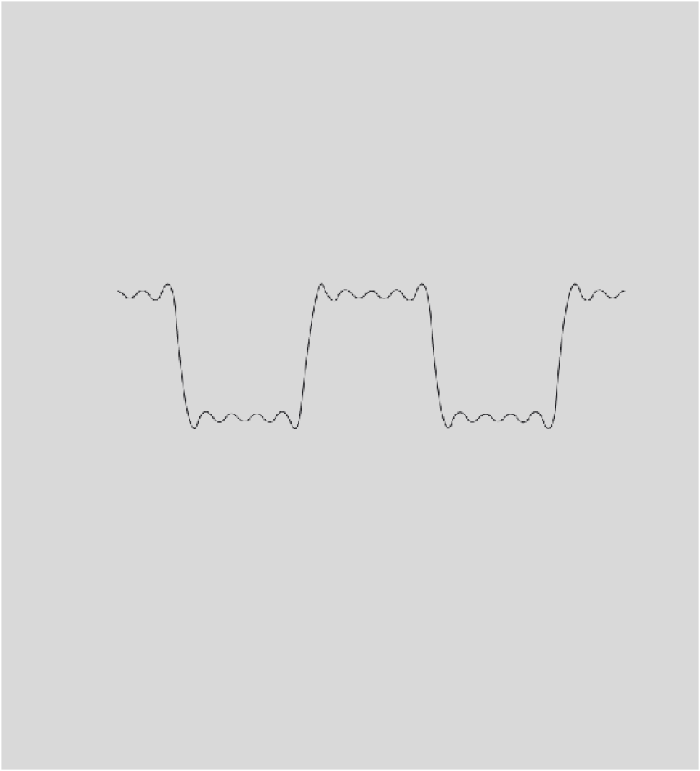
Note that the approximation of summing the first ten harmonics (Figure 11.8a) closely resem-
bles the desired square wave. The Fourier coefficients,
a
m
, for the first ten harmonics are shown as
a function of the harmonic frequency in Figure 11.8b. To fully replicate the sharp transitions of the
square wave, an infinite number of harmonics are required.
5
0
−
2
−
1
0
1
2
(a)
Time (sec)
4
3
2
1
0
−
1
2
−
0
0.5
1
1.5
2
2.5
Frequency (Hz)
3
3.5
4
4.5
5
(b)
FIGURE 11.8
(a) MATLAB result showing the first ten terms of Fourier series approximation for the square
wave. (b) The Fourier coefficients are shown as a function of the harmonic frequency.
11.5.2 Compact Fourier Series
The trigonometric Fourier series provides a direct approach for fitting and analyzing
various types of biological signals, such as the repetitive beating of a heart or the cyclic
oscillations produced by the vocal folds as one speaks. Despite its utility, alternate forms
of the Fourier series are sometimes more appealing because they are easier to work with