Biomedical Engineering Reference
In-Depth Information
Table 2.2-3 Summary results of hemispheric activation differences in 5 tests on 7 subjects from
Keirn (1988). These quantities are expressed
in percent differences between the left and right hemispheres.
Central (C3, C4)
Parietal (P3, P4)
Occipital (O1, O2)
Freq band
d
q
a
b
l
b
h
d
q
a
b
l
b
h
d
q
a
b
l
b
h
Task
Composite differences
1
1.66 0.07
1.64 2.30 6.12 0.64 0.05
1.24 1.71 2.70 0.40
1.56
4.81
1.72
2.84
2
0.72
0.75 3.86 3.60 0.35
0.97
0.39 5.59 7.35
1.67
0.70
1.71
2.09
0.76
4.60
3
1.62 1.33 4.12 3.44 1.78 0.62 0.99 1.44 2.19
0.48
0.75
2.68
6.93
4.89
5.73
4
0.83
1.13 2.49 2.64 0.38 0.60
0.54 1.42 4.87
0.32
1.89
2.09
3.33
1.27
3.74
5
0.06
0.16 1.84 2.66 2.36 0.14
0.65 1.32 3.72 0.62
0.46
1.95
4.24
2.17
0.93
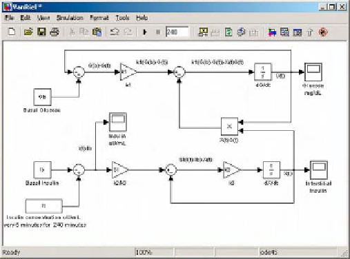
Example 2.2.4 Simulink model of glucose regulation.
Use Simulink to solve the system of equations (2.2.1)
for glucose as a function of time. Use the constants
k
1
,
k
2
and
k
3
and insulin profile
I
(
t
) from Van Riel (2004).
To use Eqs. (2.2.1), four unknowns must be de-
termined before using MATLAB or Simulink to solve
for
G(t).
Van Riel (2004) rewrites the second of
Eqs. (2.2.1) as
dXðtÞ
dt
¼ k
3
ðS
I
ðIðtÞI
b
ÞXðtÞÞ
where
S
I
¼ k
2
/
k
3
is called the insulin sensitivity.
Van Riel solves this problem using the Runge-Kutta
solver ode 4 5 in a MATLAB script. While there is
flexibility in using the script to vary the parameters or the
insulin profile, a set of MATLAB scripts and a Simulink
implementation make for easier documentation of the
different model systems. The MATLAB script for normal
glucose kinetics is
Figure 2.2-8 Simulink model of glucose regulation.
a constant for each. The Simulink model is shown in
Fig. 2.2-8
.
The key to making this simulation work is the ''From
Workspace'' block, which is in source of the insulin
profile
I
[
t
]. The source for a ''From Workspace'' block is
a 2D array, with the time points in the first column and
the values in the second. For this problem, the array is
%
% Time course of insulin I(t)
%
t_insu
¼
[0 5 10 15 20 25 30 40 60 80 100 120 140
160 180 240];
u
¼
Ib
þ
[0 100 100 100 100 00000000000];
It
¼
[t_insu' u'];
% Set the workspace variables for the
% Simulink model VanRiel.mdl
% Basal Glucose and Insulin
Gb
¼
92;
Ib
¼
11;
G0
¼
279;
% Model constants
SI
¼
5e
4;
k3
¼
0.025;
k1
¼
2.6e
2;
where the constants and insulin profile are taken from
Van Riel (2004). Notice that the constants
G
b
and
I
b
are
MATLAB variables and the initial value of the integrator
labeled dG/dt is the MATLAB variable
G
0 . The gain
boxes serve as multipliers by the constants
k
1
,S
l
and
k
3
,
respectively, rather than using a multiplier box and
Notice that the first seven samples are every five minutes
and they are spaced further apart until 240 minutes. Since
the time step of the simulator must be a constant, it is
necessary to indicate to Simulink that it must interpolate
the missing values. Also, in the event that the input is