Hardware Reference
In-Depth Information
Figure 2.18
Figure 2.19
a) Sketch, on the left, the DFF's functional response.
b) Sketch, on the right, the timing response. Assume
t
pCQ(LH)
= 2 ns,
t
pCQ(HL)
= 3 ns, and
t
pRQ
= 1 ns (the vertical lines are 1 ns apart).
Exercise 2.2: Metastability and Synchronizers
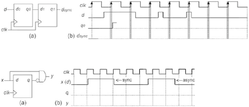
A popular synchronizer was presented in i gure 2.6b and repeated in i gure 2.18 along
with an illustrative timing diagram.
a) What do the gray areas in i gure 2.18b represent?
b) Which time parameters dei ne the aperture window's width?
c) Is it desirable that the aperture window be as narrow as possible or as wide as
possible?
d) Why must
d
remain stable during that time interval? What is metastability?
e) Why can synchronizers reduce the effect of metastability?
f) Given the asynchronous input
d
shown in the i gure, draw the waveforms for
q
0
and
d
sync
. (The initial part of
q
0
was already drawn; the delay included between the
clock edge and the signal edge is
t
pCQ(LH)
.)
g) At which positive clock edge (i rst, second, etc.) after
d
goes up does the signal
actually delivered to the FSM (
d
sync
) go up?
h) Two short pulses (lasting less than one clock period) are included in the
d
wave-
form. Are they always detected? Explain.
Exercise 2.3: Basic One-Shot Circuit
Figure 2.19a shows the same elementary one-shot circuit seen in i gure 2.10, which
must produce at the output a pulse with a i xed (one clock period) duration every
time the input goes up.