Geology Reference
In-Depth Information
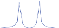
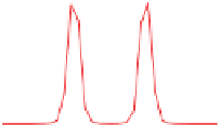
Figure 4.10
Effect of tapering
on the same test time series as
in Figure 4.9, here sampled
at Δt = 1 for N = 2048 with
two sinusoids at frequencies
f
1
= 0.050 and f
2
= 0.055. (a) The
Dirichlet-tapered test time
series (top), Bartlett-tapered
time series (middle), and
Hann-tapered time series
(bottom). (b) The
periodograms of each tapered
series is shown; arrows show
attenuation of leakage by the
Bartlett- and Hann-tapered
periodograms. The inset shows
that the Bartlett and Hann
periodograms have recovered
some of the power leaked by
the Dirichlet periodogram,
although they also fail to bring
the power to the true modulus
value of 2048. The leakage
occurs because the frequencies
do not coincide with the
frequency bins proscribed by
the FFT, although, leakage is
substantially less here, even for
the Dirichlet periodogram,
than for the example shown in
Figure 4.8, where the test time
series was much shorter, at 512
points long.
(a)
1
0
-1
1
0
Dirichlet
Bartlett
Hann
-1
1
0
-1
0
200
400
600
800
1000
Time (n)
1200
1400
1600
1800
2000
(b)
2000
2000
1500
1000
0.55
0.50
0.50
0.55
Dirichlet
Bartlett
Hann
1500
500
0
1000
0.05 0.055
Frequency (1/n)
500
0
0.01
0.02
0.03
0.04 0.05 0.06
Frequency (1/n)
0.07
0.08
0.09
0.1
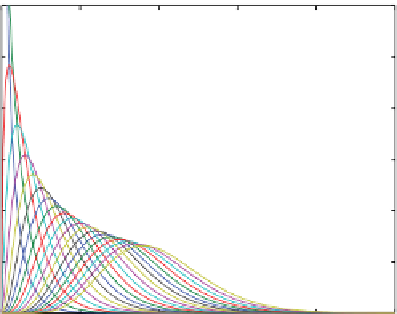
Figure 4.11
The
χ
2
distribution reported as f
n
(x)
versus x, for n = 1-20, calculated
with
chisquare.m
(Appendix).
{100(α/2)}% = 95% CLs are
listed for selected n, so that the
probability P[
χ
2
≤ lower
CL] = P[
χ
2
0.3
1
2
3
n
1
95% CL
0.2-1000
0.25
2
0.21-40
3
0.32-4
4
0.36-8.3
0.2
5
0.39-6.0
4
etc.
20
0.59-2.1
5
0.15
≥ upper CL] = α/2.
These values are used in ratio
with n, and multiplied with the
spectral estimates to obtain
upper and lower 95% CL
constraints (see example in
text). The definition of CL
constraints for spectral
estimates is required for
hypothesis testing
(Section 4.3.6).
etc.
0.1
20
0.05
0
0
10
20
30
40
50
x