Geology Reference
In-Depth Information
Time domain
Frequency domain
0
-20
1
0.8
-40
-60
0.6
-80
Dirichlet
Bartlett
Hann
-100
-120
0.4
Dirichlet
Bartlett
Hann
0.2
-140
0
10
20
30
Samples
40
50
60
0
0.2 0.4
Normalized frequency (×
π
rad/sample)
0.6
0.8
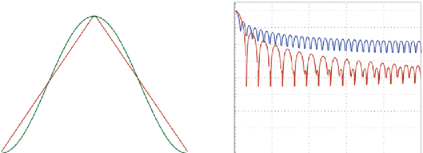
Figure 4.9
Three common data windows or “tapers” used in spectral analysis (left) and their Fourier transforms
(right). The Dirichlet (also known as the “rectangular” or “boxcar”) taper admits the entire time series from start to
finish, whereas the other two tapers strongly down-weight the beginning and ending segments of the time series.
These plots were generated in MATLAB using the Window Visualization Tool (for L = 64, wvtool(rectwin(L));
wvtool(bartlett(L)); and wvtool(hann(L)). Bartlett-tapered and Hann-tapered spectral estimates need to be corrected
by a factor of 2 (“COHERENT GAIN” column in Table 1 of Harris (1978)). The Dirichlet Fourier transform has a
central lobe with a half-power width of 0.89∆f; the Bartlett and Hann central lobes are broader at 1.28∆f and 1.44∆f,
respectively (Table 1 of Harris (1978), “3.0-dB BW (BINS)” column). The “roll-off ” of power outside of the center
lobe is -6 dB per octave with the first sidelobe at -13 dB for the Dirichlet window, -12 dB per octave with the first
sidelobe at -27 dB for the Bartlett window, and -18 dB per octave with the first sidelobe at -32 dB for the Hann
window. (Note: dB (decibels) = 10 log (P
2
/P
1
) where P
2
is power with respect to a reference power P
1
.)
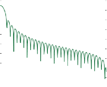
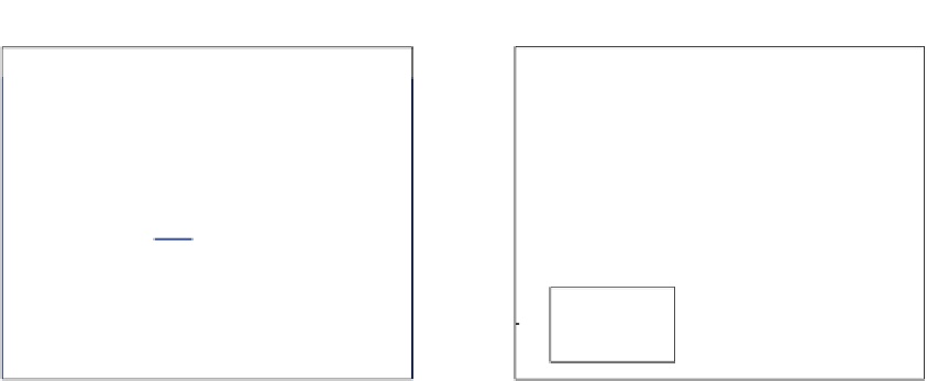
The Dirichlet window produces a spectral estimator with the narrowest
frequency resolution, but at the cost of power leakage into the sidelobes.
Leakage occurs when a true frequency component of the data time series
does not coincide with a frequency bin, as shown in Figure 4.10; the Bartlett
and Hann tapers somewhat restore leaked power back into the central lobe.
4.3.5.3 Spectral Estimator Statistics
The true strength of the spectral estimator lies in its statistics, which allows
the practitioner to interpret the data spectrum. The probability distribution
of the periodogram for Gaussian (normally)-distributed random variable
was originally described as a Rayleigh distribution (Schuster 1897). This
work laid the foundation for calculating the significance of estimated spectra
in terms of the more general
χ
2
distribution (Figure 4.11). The χ
2
distribu-
tion also provides an empirical means to determine the degrees of freedom
(dof ) n from the ratio of the mean and variance of the estimated periodo-
gram (page 22 in Blackman and Tukey (1958); page 253 in Jenkins and Watts
(1968); further information on dof bias in Elgar (1987)).
The unsmoothed (Dirichlet-windowed) periodogram is comprised of sine
and cosine functions with coefficients contributing one dof each to the
spectral estimate of a given frequency. In the FFT, the “Fourier coefficients”
are stored in a complex variable. Thus, the unsmoothed periodogram has a χ
2
distribution; the n = 2 dof can be confirmed empirically using
estdof.m