COMPUTATIONAL MODELING OF INDENTATION - Nanoindentation with Biological Applications - page 160

120

100

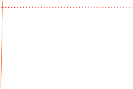
n=0.0
n=0.1
n=0.2
n=0.3
n=0.4
n=0.5

80

C
σε

60

C
σ

40

RR

r = 2· 0.0115
m = 2.0

R

Elastic limit
Plastic limit

α
ε

=°
=

70.3
0.0115

20

Eq. (9)

R

Eq. (13)

0

(c) 0 1000 2000 3000 4000

E / σε

E / σ

R R

R

Figure 6-4. The relationship between .

The numerical results (symbols) are shown with both elastic and rigid plastic limits, and
the empirical fitting function incorporating these limits is given in Eq. 6-13 (which can be
extended to other indenter angles).

C / σ and as n is varied, for α =° 70.3

E / σ R R

For a given indenter angle α , once the dimensionless loading
curvature Π is determined, if both E and ν known a priori , the only

apparent unknown variable σ can be solved numerically from the

measured P − data along with Eq. 6-5 . Next, from Eqs. 6-6 and 6-7 a
pair of flow stress-total strain (

R

) on the uniaxial stress-strain curve
can be determined from the reverse analysis as

σε ,

= = + . (6-14)
Finally, by using the dual (or plural) sharp indenter method, more
pairs of true stress-strain can be determined from the indentation analysis
when different α are used. It is commonly believed that the
dimensionless loading function Π

σσ and ε ε 2 2 σ / E

R R R

ε are
sufficiently different when another α is used. 1,53,56,73 For power-law
materials, two independent conical indentation tests with distinct apex
angle

and representative strain

R

and n
(assuming both E and ν are known); more indenter angles with larger
separation may be used and the averaged result improves the accuracy of
the reverse analysis. 5,74

α are ne ed ed to determine the plastic parameters σ

y