Infrared and Raman Spectroscopy and Imaging of Breast Cancer - Vibrational Spectroscopy for Tissue Analysis - page 139

930 cm -1 976 cm -1 1057 cm -1

1142 cm -1 1215 cm -1 1377 cm -1

1443 cm -1 1504 cm -1 1643 cm -1

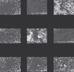
Figure 5.21 (See colour insert.)
False-colour images based on the second-derivative intensity at the indicated wave num-
bers. Blue indicates high intensity (large negative second derivative) while red indicates low
i nt e n sit y.

wavenumbers can then be plotted as images (Figure 5.21). These plots reveal
a few interesting features.

• The peaks at 1057 and 1215 cm −1 clearly contrast two regions of
the sample. They appear to be complementary to each other: high
intensity at 1057 cm −1 is correlated to low intensity at 1215 cm −1 . This
implies a significant physical difference between these two regions
of the sample.
• There is a horizontal line of pixels near the bottom of the image
that stands out, particularly at 976 cm −1 . This is presumably due to
a defect of the detector (it appears in the images of other samples
as well). Specifically, it affects rows 5-8. These rows appear to be
noisier than the rest of the pixels. A plot of the Root Mean Square
(RMS) noise levels presented in Figure 5.22 confirms this, along
with a vertical line toward the right side and a few other isolated
noisy pixels.
• There also appears to be a small region near the centre of the image
that has quite low intensity for most bands (e.g., 1643, 1504, 1142,
930 cm −1 ).

The mean spectra for the left 20 columns and right 20 columns of the image
are plotted in Figure 5.23.
It is also possible to look at the frequency distributions for the intensity at
these wave numbers.
The distributions for 1057 and 1215 cm −1 are clearly bimodal, correspond-
ing to the two regions identified in Figure 5.24. Most of the other bands
appear fairly normally distributed.