Tomographic Phase Microscopy (TPM) - Biomedical Optical Phase Microscopy and Nanoscopy - page 234

1.59

1.58

1.57

1.56

1.55

(A) (B) (C)

-8

-10

-12

-14

-16

-18

(D) (E) (F)

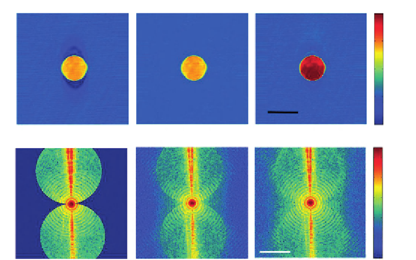
Figure. 12.6
Iterative constraint algorithm. (A) Slice image of a 6 m bead before application of the constraint

algorithm. (B) Same slice image as in (A) after application of the non-negative constraint.
(C) Same slice image as in (B) after 100 iterations. The color bar indicates the refractive indices at
633 nm wavelength. Scale bar, 5

μ

m. (D) Amplitude distribution in K x K y plane before
application of the constraint algorithm. (E) 3D Fourier transform of tomogram after non-negative
constraint. (F) 3D Fourier transform of tomogram after 100 iterations. The color bar indicates
base-10 logarithm of E-field amplitude. Scale bar, 2

μ

m 2 1 [24] . μ

polystyrene bead, we estimate that the accuracy of the measured refractive index is close to
0.001 after application of the iterative constraint algorithm. When the Fourier maps before
( Figure 12.6D ) and after ( Figure 12.6F ) iterations are compared, the ring patterns are
generated in the missing angle regions ( Figure 12.6F ). This indicates that iterative constraint
algorithm can generate reasonably accurate solutions for the missing angle regions.

To compare the performance of the inverse Radon transform and ODT, two sets of angular
E-field images are acquired for 6 m polystyrene beads (Polysciences) immersed in oil

(Cargille, n 5 1.56) at two different foci, one in the middle of the bead and the other 4

μ

μ m

above the center ( Figure 12.7 ). When the inverse Radon transform is applied, the slice
image at the middle of the bead is uniform when the objective focus is set to the middle of
the bead ( Figure 12.7A ). However, when the focus is above center, the slice image in the