GEOMETRICAL PROPERTIES OF 3D DIGITIZED IMAGES - Fundamentals of Three-Dimensional Digital Image Processing - page 94

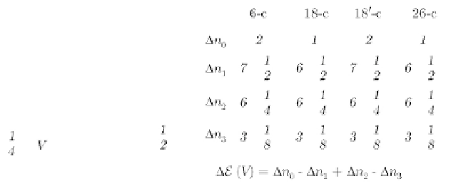
Fig. 4.12. The number of simplexes counted as in Fig. 4.11 is totaled up for each
vertex V . In the case of this figure, for example, ∆n 0 , ∆n 1 , ∆n 2 ,and ∆n 3 are added
up as in the above table.

Note that this algorithm does not depend on the type of the connectivity.
The value of ( V ) for the desired type of connectivity can be found from the

table prepared beforehand.
This method to calculate the Euler number is an extension of the method
for 2D figures given by [Gray71]. A similar method was reported in [Lobregt80]
for only the 6-c and 26-c cases based upon a closed netted surface model and
Eq. 4.8.

E

4.7.2 Simplex counting method

The Euler number is calculated by counting simplexes of each dimension con-
tained in a 3D object and substituting the results for n r s in Eq. 4.5. In the
6-c case, for example, the Euler number is calculated as shown in Fig. 4.14.

The counting of simplexes as presented above may be performed by local
template matching over a 2

E

2 local area or equivalently by calculating
a value of a pseudo-Boolean expression defined over the 2

× 2 ×

× 2 × 2 local area.

The latter procedure is presented in the following theorem.

x 7 denote density values ( 0 or 1 )of
voxels P = ( i, j, k )anditsneighbors( i + 1 ,j,k ) ,..., and ( i + 1 ,j + 1 ,k + 1 )
in the 2

x 0 , x 1 ,..., x 6 and

Theorem 4.4. Let

× × ≤ i ≤ L, 1 ≤ j ≤

2 2 local area as shown in Fig. 4.14 ( 1

M, 1 ( k )( k represents the type of the

connectivity ( k = 6 , 18 , 18 , or 26 )) of a binary image with the size L

≤ k ≤ N ). Then the Euler number E

N
is given by the following equations. Here we assume that the edge of an input
image is filled with 0-voxels [Toriwaki02a, Toriwaki02b].

× M ×

E [6] = L− 1

M− 1 N− 1

{ x 0 [ 1 − x 1 ( 1 − x 4 · x 5 )

i =2 j =2

k =2