Image Processing Reference
In-Depth Information
specified by the Fourier transform, then we should obtain the originally transformed signal.
This process is illustrated in Figure
2.4
for the signal and transform illustrated in Figure
2.3
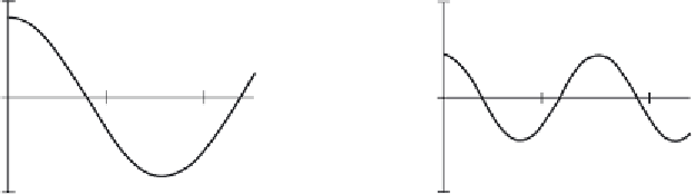
. Note that since the Fourier transform is actually a
complex
number it has real and
imaginary parts, and we only plot the
real
part here. A low frequency, that for ω = 1, in
Figure
2.4
(a) contributes a large component of the original signal; a higher frequency, that
for ω = 2, contributes less as in Figure
2.4
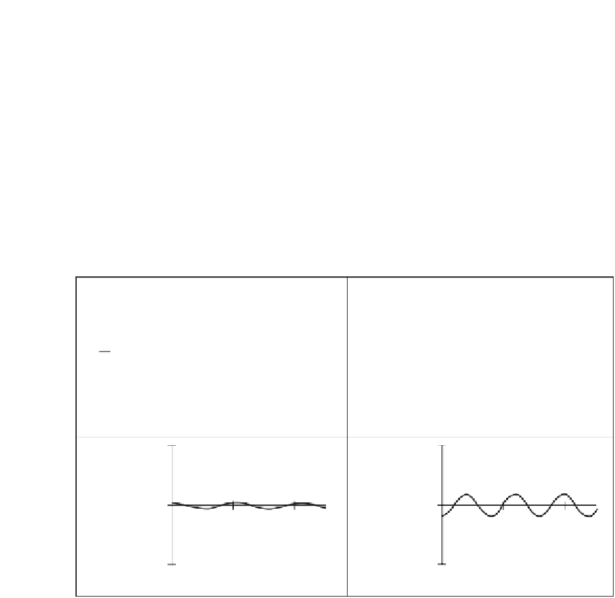
(b). This is because the transform coefficient is
less for ω = 2 than it is for ω = 1. There is a very small contribution for ω = 3, Figure
2.4
(c),
though there is more for ω = 4, Figure
2.4
(d). This is because there are frequencies for
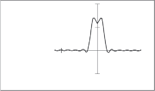
which there is no contribution, where the transform is zero. When these signals are integrated,
we achieve a signal that looks similar to our original pulse, Figure
2.4
(e). Here we have
only considered frequencies from ω
= - 6 to ω = 6. If the frequency range in integration
Re (Fp(1)·e
j·t
)
Re
(Fp(2) ·e
j·2·t
)
t
t
(a) Contribution for
= 1
(b) Contribution for
= 2
Re
(Fp(3) · e
j·3·t
)
Re
(Fp(4)·e
j·4·t
)
t
t
(c) Contribution for
ω
= 3
(d) Contribution for
ω
= 4
6
)
⋅
e
j
⋅ω ⋅
t
d
ω
Fp(
ω
-6
t
(e) Reconstruction by integration
Figure 2.4
Reconstructing a signal from its transform