Image Processing Reference
In-Depth Information
was larger, more high frequencies would be included, leading to a more faithful reconstruction
of the original pulse.
The result of the Fourier transform is actually a
complex
number. As such, it is usually
represented in terms of its
magnitude
(or size, or modulus) and
phase
(or argument). The
transform can be represented as:
pte
( )
-
jt
dt
= Re[
Fp
(
)] + Im[
j
Fp
(
)]
(2.6)
-
where Re(
) are the real and imaginary parts of the transform, respectively. The
magnitude
of the transform is then:
) and Im(
-
jt
2
2
pte
( )
dt
=
Re [
Fp
(
)]
+ Im[
Fp
(
)]
(2.7)
-
and the
phase
is:
Im[
Fp
Fp
(
)]
pte
( )
-
jt
dt
= tan
-1
(2.8)
Re[
(
)]
-
where the signs of the real and the imaginary components can be used to determine which
quadrant the phase is in (since the phase can vary from 0 to 2π radians). The
magnitude
describes the
amount
of each frequency component, the
phase
describes
timing
, when the
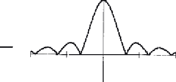
frequency components occur. The magnitude and phase of the transform of a pulse are
shown in Figure
2.5
where the magnitude returns a positive transform, and the phase is
either 0 or 2π radians (consistent with the sine function).
|
Fp
(ω
) |
arg
(Fp(
ω
))
(a) Magnitude
(b) Phase
Figure 2.5
Magnitude and phase of Fourier transform of pulse
In order to return to the time domain signal, from the frequency domain signal, we
require the
inverse Fourier transform
. Naturally, this is the process by which we reconstructed
the pulse from its transform components. The inverse FT calculates
p
(
t
) from
Fp
(ω
) according
to:
1
2
jt
pt
() =
Fp
()
e
d
(2.9)
-