Graph Visualization For Geography - Methods for Multilevel Analysis and Visualisation of Geographical Networks - page 93

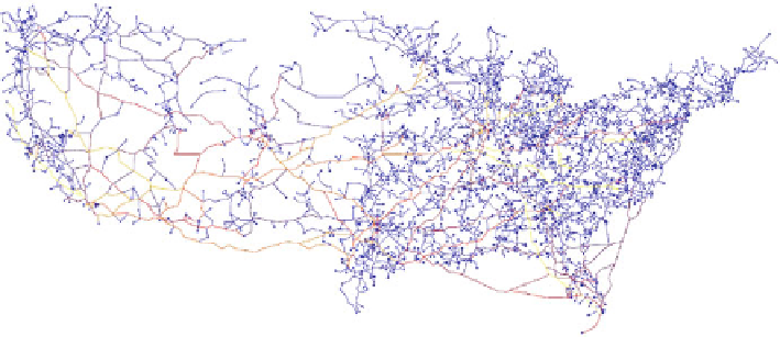
Fig. 6.9 The layout of the graph introduced in Fig. 6.8 a after the edge bundling process

transformed into larger ones. This effect is reproduced by first computing all of the
shortest paths between linked nodes on the original graph. Then, according to the
number of shortest paths through an edge of the grid, the weights of the grid edges
are adjusted. Reducing the weight of an edge is equivalent to transforming it into
a highway because it is possible to go faster from one point to another. A shortest
path for each edge of the original graph is then computed. This adjustment of the
weights creates new bundles because the new distance matrix of our graph promotes
frequently used edges. To compute the shortest paths, we use the well-known
Dijkstra's algorithm ( 1971 ), leading to O

2

( |

V grid |·| E grid | + | V grid |

· ( |

E grid | ))

log time

complexity. The result of this edge routing phase is presented in Fig. 6.9 .

6.4.3 Enhancing Edge Bundled Graph Visualization

Edge bundled graphs leverage several issues with respect to rendering the graphs on
a screen. To obtain an aesthetic drawing and to ease the retrieval of information from
the visualization, some rendering methods and visual encodings have been designed
specifically for this type of visualization technique. The following summarizes these
techniques.

Smoothing Edges with Curves

The main feature common to every edge-bundled graph visualization is the drawing
of edges as curves. Indeed, rendering graph edges as curves makes it easier to
follow the edges and gives a more visually appealing graph drawing. In 2006 ,
Holten renders bundled edges piecewise with cubic B-splines. By using this type
of spline, which provides local control of the curve shape, one can produce distinct