BLOB Analysis - Introduction to Video and Image Processing - page 108

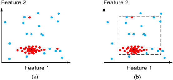
Fig. 7.8 A 2D feature space where each point is a feature vector, i.e., a BLOB. The red points are
from the object we are trying to recognize while the blue are from non-object BLOBs. ( a ) Input.
( b ) The decision region in a box classifier where the maximum and minimum values are used to
defined the decision region
Often it is not possible to define the prototype model beforehand and we therefore
need to learn it, see Appendix C. The procedure is to run the developed system on
typical input images (the more the better) and calculate the feature values for each
BLOB (both large circles and any other BLOBs that might appear in the system).
Each BLOB will result in a point in the feature space. In Fig. 7.8 (a) an example is
illustrated where the red points are from large circles and the blue points are from
other BLOBs. The task we are faced with is to figure out the decision region of
the prototype model so that as many correct BLOBs as possible are included in the
decision region and at the same time exclude as many of the incorrect BLOBs as
possible. We can see that the density of the red points is not uniform, but tends to
be higher at the center of the “point cloud” of red points, indicated by a cross in the
figure. This is a typical phenomenon independent of which features we are working
with and the center is therefore a good representation of where the prototype is
located in the feature space. The center can be calculated as the mean of all the red
points, see Eqs. 7.2 .
We can see in the figure that the red points are spread out differently in the x-
and y-direction. This is also a typical phenomenon and by analyzing how the points
are spread out we can learn the size of the decision region in Fig. 7.7 . The simplest
way is to find the minimum and maximum values of the features and let these values
define the decision region. This can, however, lead to an incorrect classification if we
have outliers . An outlier is a point that is far away from the other points in the feature
space, see Fig. 7.8 (b). A better approach is therefore is express the spreading of the
points using the variance . Like the mean, the variance is a statistical measure that
expresses something about the data. Concretely, the variance measures the average
distance the points are from the mean. So a big variance means the points are spread
out and a small variance means the points are gathered closely around the mean, see
Appendix C.