Image Processing Reference
In-Depth Information
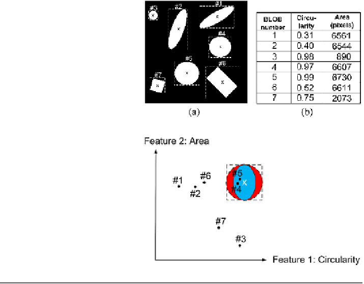
Fig. 7.6
(
a
) The figure
illustrates two features:
Bounding Box and
Center-of-Mass. (
b
) The table
illustrates two other features:
Circularity and Area. Note
the order in which the BLOBs
are labeled. This is a result of
the scan-pattern in Fig. 4.28
Fig. 7.7
2D feature space
and position of the seven
BLOBs from Fig.
7.6
(a). The
“x” represents the feature
values of the prototype. The
dashed rectangle
: box
classifier.
Red circle
:
Euclidean distance classifier.
Blue ellipse
: weighted
Euclidean distance classifier
7.3
BLOB Classification
Each of the objects in Fig.
7.6
has now been identified as separate BLOBs using,
for example, the Grass-Fire algorithm. The task is now to determine which BLOB
is a circle and which is not. As suggested above we can use the circularity feature
for this purpose. In Fig.
7.6
the values of the circularity of the different BLOBs are
listed. The question is now how to define which BLOBs are circles and which are
not based on their feature values. For this purpose we make a
prototype model
of
the object we are looking for. That is, what are the feature values of a perfect circle
and what kind of deviation will we accept? In a perfect world we will not accept any
deviations from the prototype, but in practice the object or the segmentation of the
object will not be perfect so we have to accept some deviations. For our example
with the circles, we can define the prototype to have a circularity of 1 and a deviation
of
±
0
.
15, meaning that BLOBs with circularity values in the range
[
0
.
85
,
1
.
15
]
are
accepted as circles.
What if we are looking for large circles? For this task one feature is not sufficient
and we therefore use both the circularity and the area, see Fig.
7.6
. These two fea-
tures span a 2-dimensional
feature space
as seen in Fig.
7.7
. The prototype model
will now be two dimensional with each feature having an allowed range. Together
these two ranges will form a rectangle and if a BLOB in an image has feature values
inside the dashed rectangle, then it is a large circle otherwise it is not, see Fig.
7.7
.
This approach is known as a
box classifier
and the area of the rectangle is known as
the
decision region
.