Geoscience Reference
In-Depth Information
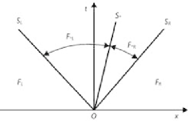
Figure 9.4
HLLC Riemann solver for
x
-split 2-D shallow water equations.
with the states
∗
L
and
∗
R
given by
⎛
⎝
⎞
⎠
1
S
∗
φ
h
K
S
K
−
u
K
=
(9.23)
∗
K
S
K
−
S
∗
K
where
is the variable representing the scalar quantity.
The wave speed estimates
S
L
and
S
R
are given by Eq. (9.19). The estimate
S
∗
for the
middle wave speed can be provided as the particle speed
u
∗
φ
that is estimated below:
1
2
(
u
∗
=
u
L
+
u
R
)
−
(
h
R
−
h
L
)(
a
L
+
a
R
)/(
h
L
+
h
R
)
(9.24)
Riemann solvers for the 2-D problem can also be established, but they are usually
very complicated. The often used method is to split the 2-D shallow water equations
(9.5) into two augmented 1-D equations along the
x
- and
y
-directions as
⎨
∂
∂
t
+
∂
F
(
)
∂
=
S
x
(
)
x
(9.25)
∂
∂
+
∂
(
)
⎩
G
=
S
y
(
)
t
∂
y
where
S
x
and
S
y
are the source terms split from
S
.
Applying the finite volume discretization scheme (9.10) for Eq. (9.25) yields
−
t
n
+
1
/
2
n
ij
F
i
+
1
/
2,
j
−
F
i
−
1
/
2,
j
)
+
t
S
xi
=
x
i
,
j
(
(9.26a)
ij
−
t
n
+
1
/
2
G
n
+
1
/
2
i
,
j
G
n
+
1
/
2
i
,
j
t
S
n
+
1
/
2
yi
n
+
1
=
y
i
,
j
(
−
)
+
(9.26b)
+
/
−
/
ij
ij
1
2
1
2