Geoscience Reference
In-Depth Information
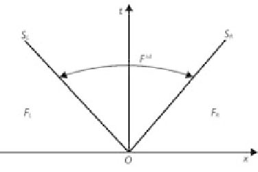
Figure 9.3
Wave structure assumed in HLL approach.
There are several ways to determine the wave speed estimates
S
L
and
S
R
. One choice
was suggested by Toro (2001) as follows:
S
L
=
u
L
−
a
L
λ
L
,
S
R
=
u
R
+
a
R
λ
(9.19)
R
where
u
K
(
K
=
L
,
R
)
is the velocity,
a
K
is the celerity, and
λ
K
is given as
⎧
⎨
⎩
1
2
(
h
∗
+
h
K
)
h
∗
if
h
∗
>
h
K
h
K
λ
=
(9.20)
K
1
if
h
∗
≤
h
K
where
h
∗
is an estimate for the exact solution of
h
in the star region and can be
evaluated as
1
2
(
1
4
(
h
∗
=
h
L
+
h
R
)
−
u
R
−
u
L
)(
h
L
+
h
R
)/(
a
L
+
a
R
)
(9.21)
The HLL approximate Riemann solver ignores intermediate waves, such as shear
waves and contact discontinuities, which arise when scalar transport equations are
added to the basic shallowwater equations. Toro
et al
. (1994) proposed a modification
of the HLL scheme to account for the influence of intermediate waves. This new
approach is called the HLLC Riemann solver. Fig. 9.4 illustrates the assumed wave
structure in the HLLC scheme.
S
∗
denotes the estimate of the speed of the middle wave.
In the exact Riemann solver,
S
. Unlike the case in Fig. 9.3, there are two distinct
fluxes in the star region in Fig. 9.4. The HLLC numerical flux is thus determined by
∗
=
u
∗
⎨
F
L
if
S
L
≥
0
F
∗
L
≡
F
L
+
S
L
(
∗
L
−
)
if
S
L
≤
0
≤
S
∗
L
F
i
+
1
/
2
=
(9.22)
⎩
F
∗
R
≡
F
R
+
S
R
(
∗
R
−
)
if
S
∗
≤
0
≤
S
R
R
F
R
if
S
R
≤
0