Biology Reference
In-Depth Information
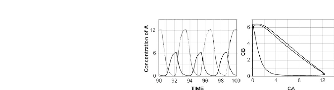
FIGURE 10-18.
Left panel: Evolution of the concentrations of hormone A (dotted) and hormone B (black), for the
model described by Eq. (10-16). Right panel: Corresponding phase diagram.
when initial estimates for the parameters are made. We saw in
Chapter 8 that providing good initial guesses for the values of the
parameters may be critical to determining the correct values of
the model parameters when nonlinear least-squares algorithms are
applied to determine the best fit between data and model. Deriving
dependencies between system parameters and experimental
observations will also facilitate our discussion of changes in sensitivity.
B. Initial Parameter Estimates
Our purpose now is to derive simple conditions, broadly linking
system parameters to experimental observations. Recall that in
deriving the mathematical form of the control function S
A
we found
a relationship between the parameters of Eq. (10-8) and the maximal
attainable hormone concentration (Exercise 10-6). Therefore, the
elimination constants
and the coefficients a and b from
Eq. (10-14) are linked with the maximal hormone concentrations in
the following way: C
A
;
max
a
and
b
¼
=a
¼
=b
. The following
result shows that, after some time (depending on the initial
conditions), the solutions will also be bounded away from zero.
a
and C
B
;
max
b
E
XERCISE
10-9
Prove that for any
as small as we like)
the following upper and lower bounds on the solution of the system
Eq. (10-14) are valid for sufficiently large t:
e >
0 (and we may choose
e
0 <
a
a
1
a
a
þ e
0
@
1
A
e
C
A
ð
t
Þ
n
B
b
þ
1
b
T
B
(10-17)
0 <
b
b
1
0
@
1
A
e
C
B
ð
t
Þ
b
=b þ e:
n
A
T
A
min C
A
þ
1