Biology Reference
In-Depth Information
from A and B can be considered random quantities and denoted by
x
and
, with the mean values of
x
and
denoted by
m
A
and
m
B
,
respectively. In this case, rejecting a null hypothesis that
m
A
m
B
will
provide evidence supporting the alternative
m
B
, which would imply
a higher yield from variety B. The null hypothesis is commonly denoted
by H
0
and the alternative hypothesis by H. In general, hypothesis
tests are classified as one-tailed or two-tailed, or, alternatively, as
one-sided and two-sided. A one-tailed test is one in which the hypothesis is
directional (i.e., uses either a ''<'' or a ''
m
A
<
''). This corn problem is an
example of a one-tailed test. In a two-tailed test, the hypothesis does not
specify a direction and will use the ''
>
'' symbol.
An example of a two-tailed test with the same data would be ''is there a
difference between the yield of plants A and B?'' In this case, the null
hypothesis would be H
0
:
6¼
m
A
¼ m
B
and H:
m
A
6¼ m
B
would represent the
two-tailed alternative.
It is important to note that the decision one makes in hypothesis testing
is to ''reject the null hypothesis'' or ''not reject the null hypothesis.'' One
does not use the language ''accept the alternative hypothesis,'' even
though this might seem appropriate. The analogy often used to explain
this philosophy is a criminal case in the United States court system,
where the null hypothesis is ''innocent'' and a jury will vote to convict
only if the evidence of guilt is compelling. A vote to acquit, therefore,
does not imply that innocence was proven.
A
0
In hypothesis testing, there are two types of error one can make. A type I
error is rejecting a true null hypothesis, and a type II error is failing to
reject a false null hypothesis. A type I error is what we really want to
avoid. In the court analogy, this would correspond to convicting an
innocent person (a type II error would be to acquit a guilty person). It is
intuitively clear that the lower we set the threshold for a type I error, the
more certain we are that we will not reject a true null hypothesis. This,
however, leads to the danger of increasing the type II error. In the
example at the beginning of this section, the probability for type I error is
the area of the shaded region in Figure 4-3(B). It is generally accepted
that this p-value should be less than 0.05 for the null hypothesis to be
rejected.
x
B
x
A
B
0
V
0
a
Back to our corn example, suppose we are testing H
0
:
m
A
m
B
versus the
alternative H
:
m
A
<
m
B
or, equivalently, H
0
:
m
A
m
B
0 versus the
C
V
1
0
V
2
alternative H
:
m
A
m
B
< 0. Suppose also that when testing our
hypothesis, we want to limit the magnitude of type I error we may be
m
aki
n
g to 0.05. From the data gathered for the experiment, we compute
x
B
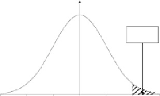
FIGURE 4-4.
Graphical representation of one-tailed and two-
tailed p-values.
. We then need to evaluate t
h
e
probability of how likely it is the sampling distribution for x
B
x
A
, which we denote by
a
x
A
,
determined assuming the correctness of the null hypothesis, would
p
rod
u
ce that value. Assume now that the sampling distribution for
x
B
x
A
is represented by the density function depicted in Figure 4-4(A).