Environmental Engineering Reference
In-Depth Information
10
2
D
L
= longitudinal diffusion coecient
d
= average soil particle diameter
v
L
= longitudinal velocity
10
1
D
L
D
o
Advection
dominant
10
0
Diffusion
dominant
Transition zone
10
-1
10
-3
10
-2
10
-1
10
0
10
1
10
2
Pe = v
L
d/D
o
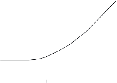
FIGURE 9.20
Diffusion and advection dominant low regions for solutes in relation to Peclet number. (Adapted from Perkins,
T.K. and Johnston, O.C.,
Journal Society of Petroleum Engineering
, 17, 70-83, 1963.)
advection-dominant transport (Figure 9.20). The longitudinal diffusion coeficient
D
L
con-
sists of both the molecular diffusion coeficient
D
m
and the hydrodynamic (mechanical)
dispersion coeficient
D
h
. This is written as
D
L
=
D
m
+
D
h
=
D
o
τ + α
v
,
where
D
m
is the molecular diffusion (=
D
o
τ;
D
h
=
α
v
), α is the dispersivity parameter, and
τ is the tortuosity factor.
The tortuosity factor is introduced to modify the ininite solution diffusion coeficient to
acknowledge that we do not have an ininite solution, and that diffusion of a single solute
species in a soil-water system is subject to constricting pore volumes and nonlinear paths.
Figure 9.20 shows that in the diffusion-dominant transport region, we can safely neglect
the
v
L
term since
v
L
is vanishingly small. Under those circumstances, the diffusion-dominant
transport region, we will have
D
L
=
D
o
τ
.
In the advection-dominant transport region, if we
consider that diffusion transport is negligible, then
D
L
= v
L
. In the transition region, the
relationship for
D
L
will be given as:
D
L
= D
o
τ
+
α
v
L
.
The signiicance of a correct choice or speciication of a diffusion coeficient cannot be
overstated. Figure 9.21 is a schematic illustration showing the variation of
D
(or
D
L
) coef-
icients calculated using Equation 2.2 in Section 2.5.4 of Chapter 2, and using the concen-
tration proiles shown at the left-hand side of the diagram in Figure 9.21. The Ogata and
Banks (1961) solution of the transport equation, similar to the one shown in Equation 2.2 in
Chapter 2 for an initial chloride concentration of 3049 ppm as the input source (Figure 9.22),
shows the different chloride concentration proiles obtained in relation to variations in the
D
value used in the calculations. The differences are not insigniicant.


Search WWH ::

Custom Search