Biomedical Engineering Reference
In-Depth Information
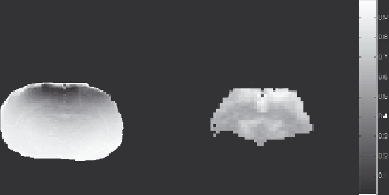
Anatomical view
H
MRI
Fig. 2.8. Spatially mapped temporal complexity of BOLD related signal across a coro-
nal section of the rat brain. The anatomical view of the brain section is seen on the
left while the corresponding Hurst exponent map calculated from a set of gradient echo
T
2
-weighted EP images is shown on the right along with an intensity coded bar of H.
The experiment was conducted on a 9.4T spectrometer (Bruker, Billerica, MA) using
a
1
H resonator/surface-coil radio-frequency probe
(36)
. Gradient echo EPI data were
acquired with
TR
=
0. 2
s. The images were collected in matrix 64×64 spatial res-
olutions; the slice thickness was 2 mm, the volume of one voxel is ∼0.15 μL. The
slice position was selected at the level of Bregma. Similar to the signals shown in
Fig.
2.1
, these signals are also of fGn class. A value of
H
<
0. 5
indicates the presence of
an anticorrelated signal,
H
=
0. 5
that of a pure random signal (i.e., no correlation),
while
H
0. 5
is associated with a correlated signal where a temporal event shows
a given degree of dependence on values preceding it. Notice that BOLD related signal
fluctuations are correlated in those areas (cortex, thalamus) where blood flow is high.
>
the brain (
Fig. 2.9
). However, for technical reasons, this is
more easily achievable with optical imaging than fMRI. Optical
reflectance imaging offers ways of mapping microregional blood
flow, and blood volume from superficial layers of such volume in
the brain cortex
(33, 34)
. When feature extraction is performed
on the map of the latter, the pial network can be traced and its
2D complexity assessed by the calculation of box dimension
(35)
(
Fig. 2.9
, right panel). The same approach can be applied in 3D
also to quantify the multi-dimensional complexity and its dynam-
ics. In this respect, lessons learned from studies aimed at defining
signal properties and evaluating fractal tools of analysis in the 2D
spatial
(35)
and 1D temporal and frequency domains can be use-
ful
(6, 14)
. Some questions that might be worth pursuing: What
voxel size can be considered adequate given current findings with
the time series data? Should anisotropy be considered as a compli-
cating factor, and if so, how can its treatment be devised? Which
of the known and tested fractal tools can be considered as candi-
dates in 3D assessment of spatial complexity? Should one attempt
to model 3D data sets similarly to the dichotomous fGn/fBm
model of time series in order to enhance selection criteria for
the analysis? These and other issues should certainly be made the
subject of future research before their detailed use in animal or
human experimentation begins.