Biomedical Engineering Reference
In-Depth Information
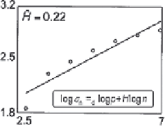
log (n)
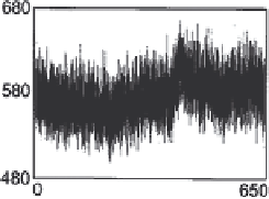
Fig. 2.3. The concept of fractal analysis as demonstrated on a time series of blood
perfusion sampled from the brain cortex by laser Doppler flowmetry. A descriptive sta-
tistical parameter, the standard deviation,
σ
, of the time series data is calculated for a
set of observation window, n.Log
σ
(n) is plotted as a function of log(n) and the fractal
descriptor is found according to the model of the scaled windowed variance method as
the regression slope across the plotted data.
Time, seconds
who provided their written consent to the study. The single and
multiple probes of the spectroscope (NIRO-500, Hamamatsu,
Japan) and the imager (courtesy of Dr. Briton Chance, Univer-
sity of Pennsylvania, PA, U.S.A.), respectively, were placed on the
forehead of the volunteers seated in an armchair.
The aim of fractal analysis is to describe, in quantitative terms,
the spatial or temporal correlation in the signals. Most of the tools
have a descriptive statistical underpinnings configured according
to the fractal concept aimed at identifying the presence of self-
similarity, as a basic fractal property, in the statistical distribution
of the data set
(6, 8)
. The novelty of the fractal approach is that
traditional statistical tools are used in a novel manner to calcu-
late descriptive statistical parameters in recursion for a range of
scales of observation (scaling range) and thus, the power-law rela-
tionship between the scales and the observed descriptive statistical
parameters (see insert in
Fig. 2.3
), becomes assessable by fitting
across the data pairs (
Fig. 2.3
).
5. Pitfalls in the
Fractal Analysis
It is crucial to realize that one cannot apply any one of the frac-
tal tools to an available signal without an assessment of the signal
variance. Fractal signals fall in two categories based on their vari-
ance
(6,14)
. If variance is time dependent, the signal is referred to
as nonstationary, while if it is not, it is called stationary. However,
the visual appearance of these signal types can be very different
in a certain resolution: the fluctuating nonstationary signal can
wander from its trend line (e.g., see signal in
Fig. 2.3
), while
the stationary signal generally fluctuates around a steady level
(e.g., see signals in
Fig. 2.1
). A precise mathematical analysis