Environmental Engineering Reference
In-Depth Information
The parameters
μ
x
,
σ
x
, and
g
x
are measures of the
average, variability about the average, and the symme-
try about the average, respectively.
In the case of bivariate probability density functions,
such as
f
(
x
,
y
), the
covariance
of the random variables
x
and
y
is commonly denoted by
σ
xy
and is defined as
0.40
m
x
= 0,
s
x
= 1
0.30
m
x
= 1,
s
x
= 2
0.20
+∞
∫
σ
=
(
x
−
µ
)(
y
−
µ
) ( ,
f x y dxdy
)
(10.15)
xy
x
y
−∞
0.10
and the variances of
x
and
y
are given by
0.00
-6
-4
-2
0
2
4
6
x
+∞
+∞
∫
∫
σ
2
=
(
x
−
µ
)
2
f x y dxdy
( ,
)
(10.16)
x
x
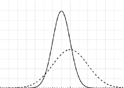
Figure 10.1.
normal probability distribution.
−∞
−∞
+∞
+∞
∫
∫
σ
2
=
(
y
−
µ
)
2
f x y dxdy
( ,
)
(10.17)
y
y
−∞
−∞
the shorthand notation n(
μ
,
σ
2
), and the shape of the
normal distribution is illustrated in Figure 10.1. Most
water-quality parameters cannot be normally distrib-
uted, since the range of normally distributed random
variables is [−∞,∞], and negative values of many water-
quality variables do not make sense. However, if the
mean of a random variable is more than three or four
times greater than its standard deviation, errors in the
normal distribution assumption can, in many cases, be
neglected.
It is usually more convenient to work with the
stan-
dard normal deviate
,
z
, which is defined by
Similar expressions for probability density functions
involving more than two random variables can also be
developed; however, such functions are not widely used
in analyzing water-quality data.
10.3 FUNDAMENTAL PROBABILITY
DISTRIBUTIONS
The analysis of water-quality data in which the measure-
ments are independent of each other is usually done
using probability distributions. In this context, the data
is first matched to a population probability distribution,
and then subsequent probabilistic analyses of the data
are done using the population probability distribution.
There are a variety of population probability distribu-
tions that are used in analyzing water-quality data. Most
of these probability distributions are derived from the
normal or log-normal distributions.
x
− µ
σ
x
z
=
(10.19)
x
where
x
is normally distributed. The probability density
function of
z
is therefore given by
1
2
2
2
f z
( )
=
e
z
−
/
(10.20)
π
10.3.1 Normal Distribution
Equation (10.19) guarantees that
z
is normally dis-
tributed with a mean of zero and a variance of unity,
and is therefore a
N
(0,1) variate. The cumulative
distribution,
F
(
z
), of the standard normal deviate is
given by
The
normal distribution
, also called the
Gaussian distri-
bution
, is a symmetrical bell-shaped curve describing
the probability density of a continuous random variable.
The functional form of the normal distribution is given
by
1
2
z
z
∫
∫
2
2
F z
( )
=
f z dz
(
′
)
′ =
e
− ′
z
/
dz
′
(10.21)
2
π
1
1
2
x
µ
σ
−
−∞
−∞
x
f x
( )
=
exp
−
(10.18)
σ
2
π
x
x
where
F
(
z
) is sometimes referred to as the area under
the standard normal curve, and these values are tabu-
lated in Appendix C.1. Values of
F
(
z
) can be approxi-
mated by the analytic relation (Abramowitz and Stegun,
1965)
where the parameters
μ
x
and
σ
x
are equal to the mean
and standard deviation of
x
, respectively. normally dis-
tributed random variables are commonly described by


Search WWH ::

Custom Search