Environmental Engineering Reference
In-Depth Information
Units of operating time
-1
Operating time
1. 3
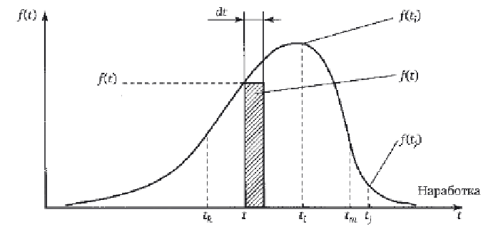
One of the possible types of graph
f
(
t
).
dt
] (geometrically this is the area of the shaded rectangle 'resting' on the
interval
dt
).
Similarly, the probability of operating time
T
fitting in the interval
[
t
k
,
t
m
] is:
t
m
{
}
∑
∫
P T t t
∈
( ,
)
≈
f t dt
( )
≈
f t dt
() ,
[1.29]
km
i
i
t tt
∈
(
)
t
i km
k
which is interpreted geometrically by the area under the curve
f
(
t
) on the
plot [
t
k
,
t
m
].
Failure probability and c.d.f. can be expressed as a function of p.d.f..
Since
Q
(
t
) =
P
{
T
<
t
}, then using the expression [1.29]
t
{
}
{
}
∫
Q t P
()
= <<= ∈
0
T t P T
(0, )
t
f t dt
() .
=
[1.30]
The extension of the interval to the left to zero is due to the fact that
T
cannot be negative.
Because
P
(
t
) =
P
{
T
≥
t
}, then
0
∞
{
}
∫
P t P t T
()
=
≤ <∞ =
f t dt
() .
[1.31]
It is obvious that
Q
(
t
) is the area under the curve
f
(
t
) to the left of
t
,
and
P
(
t
) is the area under
f
(
t
) the right of
t
. Since all values of the operating
time obtained by testing lie under the curve
f
(
t
), then
t
∞
∞
= +
t
[1.32]
Statistical estimation of failure rate (FR), expressed in units of inverse
operating time, is defined by the ratio of the number of objects ∆
n
(
t, t +
∫
∫
∫
f t dt
()
f t dt
()
f t dt Q t P t
()
=+=
()
()
1.
0
0
t

Search WWH ::

Custom Search