Biomedical Engineering Reference
In-Depth Information
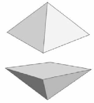
Figure 5.
Neighbouring pyramids (left) that are joined together and which, after splitting
into four parts, give tetrahedra of our 3D grid. We can the see intersection of one of these
tetrahedra with the bottom face of the voxel co-volume (right). See attached CD for color
version.
every
co-volume p
is bounded by the planes
e
pq
that bisect and are perpendicular to
the edges
σ
pq
,q
C
p
. By this construction, if
e
pq
intersects
σ
pq
in its center, the
co-volume mesh corresponds exactly to the voxel structure of the image inside the
computational domain Ω where the segmentation is provided. Then the co-volume
boundary faces do cross in NDF nodes. So we can also say that the NDF nodes
correspond to zero-measure co-volumes and thus do not add additional equations
to the discrete model (cf. (10)), and they do not represent degrees of freedom in
the co-volume method. We denote by
∈
E
pq
the set of tetrahedra having
σ
pq
as an
edge. In our situation (see Figure 4), every
E
pq
consists of 4 tetrahedra. For each
∈E
pq
, let
c
pq
be the area of the portion of
e
pq
that is in
T
, i.e.,
c
pq
=
m
(
e
pq
∩
T
T
),
where
m
is a measure in
IR
d−
1
. Let
N
p
be the set of all tetrahedra that have a DF
node
p
as a vertex. Let
u
h
be a piecewise linear function on
T
h
. We will denote a
constant value of
|∇
u
h
|
on
T
∈T
h
by
|∇
u
T
|
and define regularized gradients by
u
T
|
ε
=
ε
2
+
|∇
|∇
u
T
|
2
.
(9)
We will use the notation
u
p
=
u
h
(
x
p
), where
x
p
is the coordinate of the DF node
p
of
T
h
.
With these notations, we are ready to derive co-volume spatial discretization.
As is usual in finite-volume methods [59, 58, 57], we integrate ((8)) over every
co-volume
p,
ı=1
,...,M
. We get
.
g
0
dx.
u
n
−
u
n−
1
τ
∇
u
n
1
dx
=
p
∇
(10)
|∇
u
n−
1
|
|∇
u
n−
1
|
p