Results - Response of Flood Events to Land Use and Climate Change - page 160

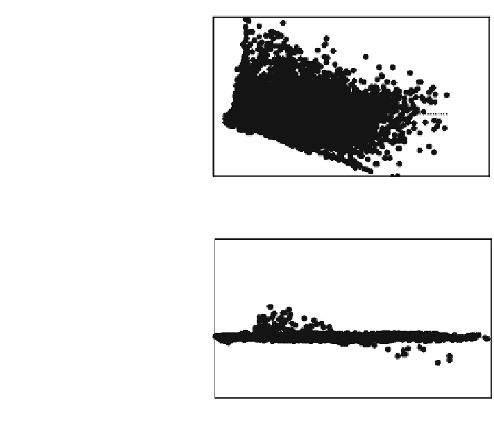
Fig. 6.27 Linear regression
analysis for residual values.
a Comparison between DEM
5 m and DEM 10 m before
resampling; b comparison
resampling DEM 5 m and
DEM 10 m after resampling

(a)

Estimate x Residuals

500
400
300
200
100
0
-100
-200
-300

1,100 1,200 1,300 1,400 1,500 1,600 1,70

Estimated

(b)

Estimate x Residuals

500
400
300
200
100
0
-100
-200
-300

1,100 1,200 1,300 1,400 1,500 1,600 1,700

Estimated

sampled data points between a dependent variable (DEMs 10 m before (a) and
after (b) resampling) and an independent variable (DEM with 5 m resolution). As
shown in Fig. 6.26 a and b, the estimated and residual values are better fitted with
the values of DEM 5 m and a linear regression is statistically significant. Fig-
ure 6.27 shows linear regression analysis for residual values. a. Comparison
between 5 and 10 m before resampling; b. comparison between 5 and 10 m after
resampling.
A further characterization of the data includes skewness and kurtosis. To this
propose, the standard residual diagnosis graphs, including the histogram of the
residuals was plotted which seems to be normal in both models in Fig. 6.28 a and b.
The skewness values for DEMs before and after resampling are equal to 1.14 and
4.11. It seems that the skewness for DEM before resampling is symmetry or
precisely, because it looks same to the left and right of the center point. Positive
values for the skewness indicate data that are skewed right. Skewed right, means
that the right tail is long relative to the left tail.
The Kurtosis value for resampled DEM showed high Kurtosis tend to have a
distinct peak near the mean, decline rather rapidly, and have heavy tails. Dataset in
DEM before resampling indicated low kurtosis tend to have a flat top near the
mean rather than a sharp peak (Fig. 6.28 ).