Results - Response of Flood Events to Land Use and Climate Change - page 159

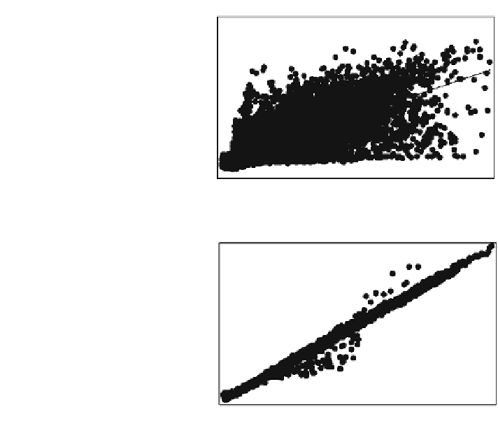
Fig. 6.26 Linear regression
analysis for estimated values.
a Comparison between DEM
5 m and DEM 10 m before
resampling; b comparison
between DEM 5 m and DEM
10 m after resampling

(a)

DEM5m x Estimate

1,700

1,600

1,500

1,400

1,300

1,200

1,100

1,100 1,200 1,300 1,400 1,500 1,600 1,700

DEM5m

(b)

DEM5m x Estimate

1,700

1,600

1,500

1,400

1,300

1,200

1,100

1,100 1,200 1,300 1,400 1,500 1,600 1,700

DEM5m

• Mean error presents the arithmetic mean of the error values and reveals whether
the interpolation has a tendency to under or overestimate on average.
• Standard deviation shows how much variation or ''dispersion'' there is from the
average. A low standard deviation indicates that the data points tend to be very
close to the mean, whereas high standard deviation indicates that the data points
are spread out over a large range of values.
• ''Residuals'' are defined as meaning the spatially modeled component of vari-
ation not accounted for by the environmental variables, and that is why it has a
very strong spatial structure (because it is added when modeling the semi-
variogram). By doing this, it is 'released', at the same time, the effect of the
spatial structure.

As shown in the Table 6.14 , mean error in both modeling results is p value
\.001. Other estimation results show that DEM 10 m after resampling was in
better agreement with the original high resolution DEM. Furthermore, the esti-
mated values are close to the 5 m DEM resolution values. The next analysis refers
to distribution of the estimated and residuals values between DEM 10 m (before
and after resampling) and DEM 5 m. Figure 6.26 a and b shows the linear
regression analysis which is modeled on the relationship between 10,000 randomly