Chemistry Reference
In-Depth Information
L
2
L
2
E
2
E
2
x
2
x
2
E
E
x
1
x
1
0
E
1
L
1
0
E
1
L
1
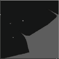
(a)
(b)
Fig. 1.12
The Cournot oligopoly with linear demand/quadratic cost. Firms use partial adjustment
towards the best response. Basins of attraction of the various equilibria for different values of the
number of firms N.(
a
) The 3-firm case. Here both E
1
and E
2
are stable.
Dark grey
basin of E
2
;
light grey
basin of E
1
.(
b
) The 5-firm case. Now E
1
is stable, E
2
is unstable.
Light grey
basin of
E
1
;
white
basin of the two cycle
of the two boundary equilibria E
1
and E
2
for N
D
3 firms. To guarantee non-
negative prices, we have selected L
1
D
7 and L
2
D
L
3
D
4. Both boundary
equilibria are asymptotically stable, each with its own basin of attraction represented
by the different shadings of grey. In Fig. 1.12b we show the situation for N
D
5
firms where L
1
D
7 and L
2
D D
L
5
D
2. Now only the boundary equilibrium
E
1
is asymptotically stable, and its basin is represented by the light grey region.
Points located in the white region converge to the 2-cycle represented by the two
dots.
1.3.3
Cournot Duopoly Revisited: A Gradient Type
Adjustment Process
The local stability of an equilibrium and the global dynamics depend on the
adjustment mechanism the firms use to update their production choices. We now
reconsider the duopoly case analyzed in Sect. 1.3.1, but instead of assuming partial
adjustment towards the best response, we now consider a discrete time adjustment
process based on marginal profits, similar to the gradient adjustment process dis-
cussed in Sect. 1.2 (1.32). However we assume now that the
relative
variation in
production quantities is proportional to the marginal profits, that is firm i adjusts its
output according to
D
a
i
@'
i
@x
i
x
i
.t
C
1/
x
i
.t/
x
i
.t/
with a
i
>0. With these assumptions, the dynamics are now governed by the discrete
time system

Search WWH ::

Custom Search